How To Interpret Marginal Willingness To Pay
A pricing lead deciding whether to ship a feature at a premium is really asking how to interpret a marginal willingness-to-pay (WTP) number from a conjoint study. Read it as a price only when it carries three things: a confidence interval built on the experiment's randomized design, a competitive-choice context, and a discount for the gap between what people say they'd pay and what they actually pay. A bare coefficient ratio, the attribute coefficient divided by the price coefficient, has none of the three and is not a price yet.
- The standard ratio-of-coefficients WTP estimator can have an undefined standard error, because the price coefficient's own sampling distribution can span zero (ScienceDirect, 2023).
- Algebraic WTP calculations that ignore competitive alternatives and the "None" option systematically overstate what customers will pay (Sawtooth Software).
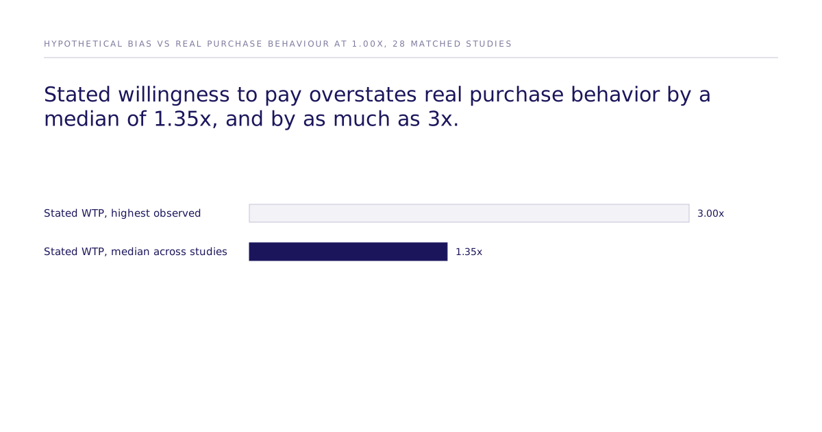
- A meta-analysis of 28 matched hypothetical-and-real-payment studies found stated WTP overstates real purchase behavior by a median of 1.35x, and as high as 3x in some studies (Environmental and Resource Economics, 2005).
- The same choice data can produce materially different WTP numbers depending on whether the model is specified in preference space or WTP space.
- A defensible WTP figure needs a delta-method or bootstrap confidence interval, a simulation against a named competitive set, and an explicit hypothetical-bias discount, not a single point estimate.
What a marginal WTP number actually captures
A marginal WTP estimate comes out of a discrete choice model, usually McFadden's multinomial logit, Mixed Logit, or an Integrated Choice and Latent Variable (ICLV) model, fit to a set of randomized product-profile choices. The analyst takes the coefficient on the attribute of interest and divides it by the (negative) coefficient on price. The result is read as "the dollar amount customers will pay for this feature." That reading assumes the ratio behaves like an ordinary number with a stable variance. It doesn't, because it's a ratio of two estimated quantities, not a directly estimated quantity itself. DCE, Mixed Logit, and ICLV are estimators for recovering these coefficients from choice data; the causal claim in a WTP study comes from the randomized manipulation of attributes in the experiment design, not from the estimator itself.
Why the standard ratio has no valid confidence interval
A WTP figure earns trust only when its limits ship with it. The price coefficient is estimated with sampling error. That error can put real probability mass on both sides of zero. Divide by it, and the result behaves like a Cauchy distribution: undefined variance, sometimes bimodal, sometimes with no meaningful mean. Hensher and colleagues showed in 2023 that the naive ratio estimator has no valid standard error under standard assumptions unless the cost parameter is reparameterized, for example with an exponential transform that forces it to stay negative (ScienceDirect, 2023). A WTP figure reported without a delta-method or Krinsky-Robb confidence interval isn't a conservative simplification. It's a number whose error bars, if computed honestly, might not exist in the form the report implies.
Why does WTP inflate without a competitive set?
Naming this failure mode is what lets a buyer check the number before pricing off it. WTP inflates because a ratio calculated from two attributes in isolation ignores that a real buyer is choosing among competing products, including the option to buy nothing at all. Sawtooth Software's technical papers on this problem show that traditional algebraic and two-product WTP calculations systematically overstate willingness to pay, because they never force the simulated respondent to weigh the feature against real alternatives or a "None" option. Sawtooth's recommended fix is to simulate share-of-preference against a full competitive set and bootstrap the resulting confidence interval, rather than solving the ratio algebraically (Sawtooth Software). That kind of share-of-preference simulation is typically built on a logit model, which carries the independence of irrelevant alternatives (IIA) assumption: adding or removing one competitor shouldn't change the relative odds between two others. When that assumption doesn't hold, for example when two competitors are close substitutes, a flat logit share simulation will misstate how share actually moves, and Mixed Logit is the standard correction.
How much should you discount stated WTP for hypothetical bias?
This gap gets published so a buyer can judge the number before acting on it. Treat a stated WTP figure as running about a third higher than what customers would actually pay at the median, and up to three times higher in some studies, unless the survey design is incentive-aligned. A meta-analysis of 28 stated-preference studies that compared hypothetical and real-payment elicitation for the same goods found a median ratio of hypothetical-to-actual value of 1.35, meaning stated WTP overstates real purchase behavior by about a third on average, with some studies in the sample running as high as 3x (Environmental and Resource Economics, 2005). This is on top of, not instead of, the confidence-interval and competitive-set problems above.
Why the same data can produce two different WTP numbers
This split is spelled out here so a buyer comparing two vendors' numbers knows which model produced each one. Two analysts can run the identical choice data through two legitimate model specifications and get materially different WTP distributions, because WTP can be estimated in "preference space," where you estimate ordinary utility coefficients and then divide, or in "WTP space," where the price sensitivity is reparameterized so WTP is estimated directly. Kenneth Train and Melvin Weeks showed in "Discrete Choice Models in Preference Space and Willingness-to-Pay Space" (2005) that the two specifications do not converge on the same WTP distribution from the same choices, because the distributional assumptions placed on the coefficients differ between the two parameterizations. Neither model is wrong; they encode different assumptions about how price sensitivity varies across the population, and a buyer comparing two vendors' WTP numbers should ask which specification produced each one.
| Naive ratio (uncorrected) | Preference-space model | WTP-space model | |
|---|---|---|---|
| What's estimated directly | Utility coefficients, WTP computed after the fact | Utility coefficients, WTP computed after the fact, with delta-method or bootstrap correction | Price sensitivity distribution, WTP estimated directly |
| Confidence interval | Usually none reported; often undefined if computed honestly | Valid, via delta method or Krinsky-Robb | Valid, but sensitive to the assumed WTP distribution |
| Common failure mode | Cauchy-like, sometimes bimodal WTP with no real mean | Still ignores competitive context unless simulated separately | Can produce implausible tails if the distributional assumption is wrong |
| Best for: | Nobody. Should not ship as a pricing input. | Buyers who want interpretable attribute-level coefficients alongside a defensible interval | Buyers who want a directly modeled price-sensitivity distribution and can validate the distributional assumption |
What a defensible WTP figure requires
A defensible WTP figure requires three things reported together: a confidence interval from the delta method or bootstrap (Krinsky-Robb), a share-of-preference simulation against a named competitive set that includes a "walk away" option, and an explicit discount or caveat for hypothetical bias.
ISPOR's Good Research Practices Task Force reports on conjoint analysis, published between 2011 and 2016, formalized the delta-method and Krinsky-Robb correction methods for health-economics discrete choice experiments. A point ratio without a valid interval isn't a publishable result in that field, and it isn't a defensible pricing input in any other.
How does a causal experiment change what a WTP number means?
It changes what the confidence interval is allowed to claim. A WTP interval from a randomized experiment covers the effect within the simulated population that was run, not the real market unconditionally. And a simulated choice is still a stated preference, not a purchase: any WTP figure that comes out of one should be discounted and reported with its interval, not treated as a bare number.
Subconscious runs randomized experiments, analyzed with discrete choice models such as McFadden discrete choice, Mixed Logit, and ICLV, on a simulation of the market, and validates the resulting studies against real human behavior. Our best configuration reaches 87% of the measured human ceiling on one study: 0.832 rank correlation against the published human result, where two independent samples of real humans reach 0.959. Across all 43 studies that pass design filters the mean is 0.73, reported in the causal fidelity paper. That's a validation-set result, not a guarantee for a new market you haven't tested, and because published human studies can sit in a model's training data, the replication protocol is built to control for that risk rather than assume it away.
The current results across studies are public on the leaderboard. None of this removes the hypothetical-bias problem named above. More on how the validation protocol works is in the methods and validation hub.
If you're evaluating a vendor's WTP output, ask for three things before you price anything off it: the confidence interval and how it was derived, the competitive set the share simulation ran against, and whether the number is stated or incentive-aligned. If a vendor can't produce any of the three, treat the figure as a ranking signal, not a price. For a closer look at how a specific WTP study was built and validated, book time with the team.