Gaussian Process Geospatial Modeling: Beyond Hierarchical Models
A data science or research lead evaluating a causal experimentation vendor needs to know whether the vendor's model treats geography or segments as related, or as unrelated categorical buckets. The distinction matters the moment a decision extrapolates past the regions or segments with direct data: a model that assumes no relationship between neighboring groups gives the same flat, wide-uncertainty prediction for every untested region and fails to narrow that uncertainty where nearby evidence exists, a direct risk for pricing, messaging, or launch calls that extend beyond tested markets.
Why categorical grouping breaks down at the edges
A common modeling instinct treats geographic region, or any segment, as a categorical variable: observations from the same group share a group-level feature, and that feature explains within-group similarity. The flaw shows up at the boundary. A hierarchical model that groups by county, or by customer segment, shrinks every group toward the same overall mean, but treats a location or segment just across the line from a tested one no differently from one far away. Physical, social, and economic processes that generate this kind of data do not respect administrative or segment boundaries; they vary continuously.
A Gaussian process (GP) encodes a different prior: nearby observations should be similar, and that similarity should decay with distance rather than vanish at a category line.
What does the radon case study demonstrate?
The clearest public demonstration of this behavior comes from a Minnesota radon dataset (Gelman & Hill, 2006): 919 household radon measurements across 85 of Minnesota's 87 counties. A standard hierarchical approach, used in PyMC's own multilevel modeling case study, treats county as a grouping variable and shrinks each county's intercept toward a common state mean. That approach has no way to relate a county's expected value to its neighbors'.
A geospatial GP model replaces the county random effect with a spatially correlated GP draw, using a Matérn-3/2 kernel built on chordal distance (the straight-line distance between two points through the Earth's interior, computed by converting longitude/latitude to 3D Cartesian coordinates) rather than plain Euclidean distance, since raw latitude and longitude coordinates are not Euclidean on a sphere. PyMC supports this by subclassing its Stationary covariance class and overriding the distance calculation; the PyMC covariance kernel API documents the built-in kernels this extends. The kernel takes the form:
k(r) = (1 + \sqrt{3} \cdot r) \cdot \exp(-\sqrt{3} \cdot r)where r is the chordal distance between two points, scaled by a fitted length-scale parameter. In this case study, the length scale carries a prior centered at 200 km with a standard deviation of 50 km, reflecting an expectation that counties within a few hundred kilometers share similar radon levels.
Fit on the observed counties, the model recovered a southwest-to-northeast radon gradient across Minnesota and used it to generate predictions for 39 untested locations in total: the 2 Minnesota counties with no direct measurements, plus 37 bordering counties across state lines, none of them arbitrary extrapolations to a flat state average.
Where does prediction uncertainty come from?
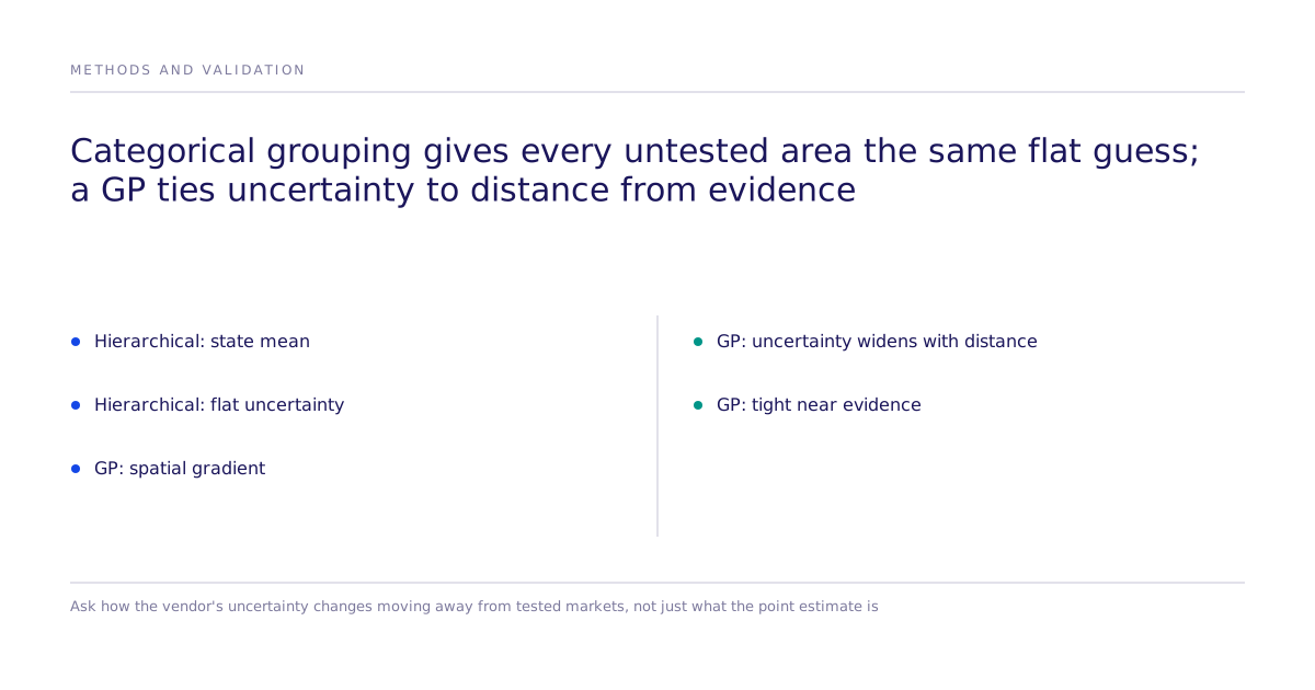
The result that matters for a buyer evaluating a vendor's modeling discipline is not the point prediction, but what happens to the uncertainty around it. In this case study, posterior predictive standard deviation stayed small within Minnesota, where observations are dense. The two unobserved Minnesota counties also kept tight uncertainty, because they sit surrounded by measured neighbors. Uncertainty widened progressively for counties farther into neighboring states, tracking distance from the training data rather than jumping to a flat, uninformative value outside the observed set.
A naive hierarchical model cannot make that distinction. Its posterior predictive uncertainty stays the same width for any unobserved group, no matter whether that group sits next to dense evidence or far away from it.
| Property | Naive hierarchical model | GP geospatial model |
|---|---|---|
| Relationship among groups | Assumes groups are interchangeable, with no correlation between them | Models correlation directly, weakening as distance grows |
| Prediction for an unobserved group | State mean, full posterior uncertainty | Spatially informed, distance-responsive uncertainty |
| Extrapolation beyond the observed region | Falls back to the state mean | Smooth extension of the learned spatial pattern within the fitted ~200 km length scale, reverting toward the mean beyond it |
| Uncertainty for an unobserved group | Constant regardless of location | Narrows near evidence, widens with distance |
The underlying discipline applies past geography
The same discipline generalizes past latitude and longitude. Any vendor's causal experiments face the same question for segments or markets with thinner direct coverage: does a result for one tested segment inform a related, untested segment, or does the model treat every untested group as a blank slate? Subconscious's causal experiments estimate effects with quantified uncertainty for the segments actually tested, rather than resetting to an uninformative default outside direct coverage. See research and the leaderboard for how that uncertainty is reported across studies, and how we work for the process from a tested segment to a broader read.
Limitations
This is one open tutorial built on one public dataset and one specific kernel choice; it is not a benchmarked or replicated production capability claim, and it says nothing about the internal architecture, accuracy, or deployment specifics of any particular vendor's model, including Subconscious's. The model itself also omits the radon dataset's basement/floor indicator for simplicity, which its own documentation flags as a natural extension rather than a finished result.
What to check before trusting a vendor's regional or segment claims
Before trusting any vendor's regional or segment-level effect estimate, ask what happens to its confidence interval outside the tested set: does it stay artificially tight and constant everywhere, or does it widen as coverage thins out? A model whose uncertainty does not respond to distance from evidence is making the same error a naive hierarchical model makes with county boundaries, just with a market map instead of a state map.