Why a Confounder Can Make a Marketing Channel Look Effective When It Isn't
A marketing team sees sales rise whenever Google Ads run. The obvious read is that the ads work. The obvious read can be wrong, and a worked Bayesian example shows exactly how.
The setup: two channels that move together
The team runs TV campaigns and Google Ads together. When TV is live, Google Ads are usually switched on; when TV is off, Google Ads are usually switched off to conserve budget, though the coordination isn't perfect. That coordination is the problem. If TV independently drives sales, then Google Ads will appear to drive sales too, even if Google Ads contribute nothing on their own.
This is a confounder: a variable that causally influences both the treatment (Google Ads) and the outcome (sales), producing a correlation between the two that has nothing to do with a direct causal link.
How is the causal structure built?
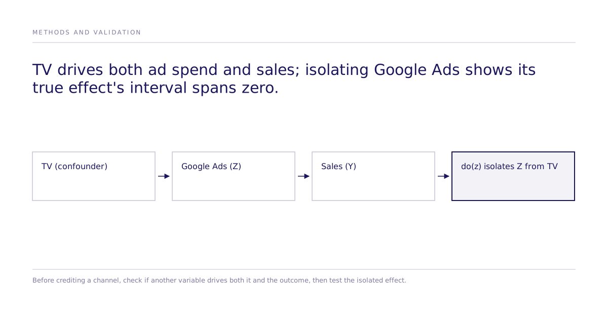
The example maps the scenario to three variables: C (TV, the confounder), Z (Google Ads on/off), and Y (sales). TV influences both Z and Y. The analysis isolates how Z acts on Y on its own, stripped of the raw correlation between Google Ads and sales.
Two regressions encode this structure: a logistic regression of Google Ads on TV status, and a linear regression of sales on TV and Google Ads. This directed acyclic graph is the model's explicit statement of what causes what, the only thing that makes the later estimate interpretable as causal rather than merely predictive.
How is the model tested against a known answer?
Before trusting any real-world estimate, the analysis simulates data from the same structure with the true causal effect of Google Ads on sales set to exactly zero. This is a parameter-recovery check: if a model can't recover a known answer on data built to match its own assumptions, it has no business estimating an unknown one.
A naive look at the simulated data, comparing sales when Google Ads were on versus off, shows a large, visually convincing gap between the two groups. The true causal effect is zero. The entire apparent gap is TV's doing.
PyMC's new do operator makes the counterfactual comparison possible inside a standard probabilistic model. It fixes a variable to a specific value and severs it from the variables that would normally influence it, the mechanics behind asking "what would sales have looked like if Google Ads had been forced on, or forced off, independent of TV?" Applied here, do(z=0) and do(z=1) generate two counterfactual sales distributions with TV pinned to its observed values. The Average Treatment Effect (ATE) is the difference between them, and in the simulation the model's posterior concentrates near the true value of zero, with the interval covering it.
For the code walkthrough, covering the generative model, the do() calls, and the posterior sampling, see the source do-operator example and the related excess-deaths counterfactual example from PyMC.
What does the estimate look like once it's real?
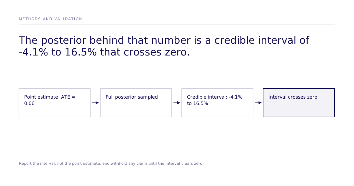
With the model validated on known data, the same procedure runs on the (still simulated, but now "observed") dataset without knowing the true effect in advance. The estimated ATE comes out at 0.06, small and positive. A point estimate alone would tempt a naive analyst to credit Google Ads with a real, if modest, lift.
The full posterior tells a different story: the credible interval for the ATE spans zero. Scaled against TV's own effect, Google Ads shows a posterior median of 6.2% relative to TV's effect, with a credible interval of -4.1% to 16.5% that includes zero, so no directional effect is supported.
The practical argument here is for reporting full uncertainty rather than collapsing it into a single threshold verdict. A 2019 commentary in Nature made a related point about statistical-significance thresholds more broadly: dichotomizing results at a significance cutoff encourages false confidence in exactly this kind of ambiguous result.
What this generalizes to, and what it doesn't
Real marketing budgets span more than two channels, and the same logic scales: higher-funnel spend like TV builds awareness over time, lower-funnel spend like paid search acts closer to the point of purchase, and confounders can sit at multiple levels of that funnel. Media Mix Models formalize this at scale, adding saturation and time-delayed adstock effects on top of the same causal reasoning.
But the method has a hard limit: a posterior estimate like this one is only as trustworthy as the DAG it's built on. Get the confounder structure wrong, miss a variable that influences both treatment and outcome, and the model will produce a confidently wrong ATE with a narrow, reassuring-looking credible interval. This single simulated example demonstrates the mechanism; it doesn't establish that any particular real-world estimate built this way is accurate. Parameter recovery on simulated data validates that the model works as intended, not that the assumed causal graph matches the real world.
Beyond one model per question
The do-operator example is a single structural causal model, hand-built around one specific DAG, answering one specific question about two channels. That is real, careful work, and it's also the pattern's limit: every new causal question needs its own model, its own DAG, and its own parameter-recovery check.
Subconscious sits a step above that per-question modeling work. Once a team has identified the causal question, does this action change this outcome for this population, Subconscious runs a randomized controlled experiment, using McFadden MNL, mixed logit, or ICLV, that compares the specific actions directly, on a simulated population, and reports the effect with quantified uncertainty, without requiring a bespoke structural causal model like the DAG above to be hand-built for each new question. The research program and replication leaderboard document how those effect estimates get checked against outcomes. Where a question benefits from moving past simulation, the how-we-work overview covers testing against real human participants without changing the causal question being asked.
The lesson from the confounder example holds either way: a number that moves in the direction you hoped for is not evidence until you've asked what else could have produced it.