Why a Single-Number Forecast Hides the Decision You're Actually Making
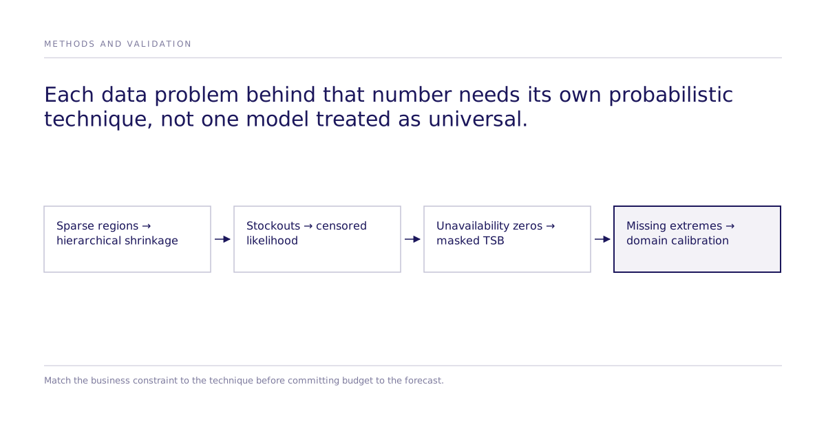
A demand forecast that returns one number is answering a question nobody asked. Inventory, pricing, and budget decisions depend on a range of plausible outcomes and how likely each one is, not a single point that erases the uncertainty around it. Probabilistic forecasting methods model the full outcome distribution instead, and five common data problems show why that distinction changes the decision.
Why does sparse per-region data understate the trend?
When a business forecasts hundreds of related series at once, such as sales by state, region, and product category, the smaller groups often carry too little history to estimate a trend on their own. Fitting each series independently treats that sparsity as noise rather than as a signal that can be borrowed from related series.
Hierarchical models address this by sharing information across the group structure, a regularizing effect known as shrinkage. In a tourism-demand example spanning 308 combinations of state, region, and travel purpose from 1998 to 2016, an independently fit model missed a mild trend component in the smaller regions that a hierarchical model recovered from the shared structure (Forecasting: Principles and Practice). The result is not automatic: strong single-series baselines are hard to beat, so establishing one before layering in hierarchy remains good practice.
Why do stockout-censored sales understate true demand?
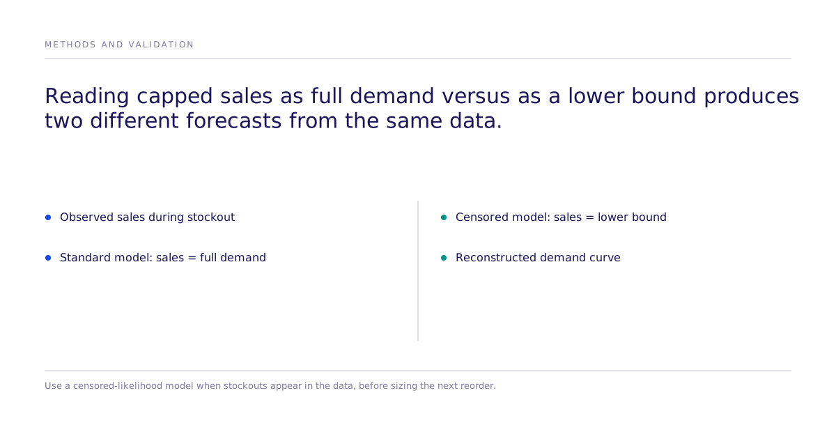
Retail sales data only records demand while a product is in stock. Once inventory runs out, the recorded sales figure is capped, or censored, at whatever was available to sell, not the true unconstrained demand for the rest of that period.
A model that treats observed sales as the complete signal will systematically underestimate future demand, because it never learns what would have sold absent the stockout. A censored-likelihood model treats observed sales as a lower bound rather than the full truth, which lets it reconstruct the unconstrained demand curve through periods with stockouts or capacity limits, keeping undercounted demand from compounding into the next reorder.
Why do unavailability-driven zeros get mistaken for no demand?
Most items in a retail catalog do not sell every day. For products with sporadic demand, a standard intermittent-demand model such as Teunter-Syntetos-Babai (TSB) cannot tell the difference between a true zero (no customer wanted it) and a zero caused by the product being unavailable to buy.
Extending the model with an availability mask corrects this: it keeps the estimated probability of demand from collapsing just because recent days happened to be out of stock. A product with two consecutive zero-sales days due to unavailability still gets a non-zero forecast once availability returns, instead of the more sharply depressed forecast a standard model would produce by treating unavailability zeros as true zeros.
Missing extreme-case data leaves edge cases unconstrained
Historical data rarely covers every condition a forecast needs to handle. An electricity-demand model built only on observed temperatures, for example, has little information about how demand behaves at extremes the data barely touched.
Calibrating the model with domain knowledge, such as the physical expectation that demand rises sharply above roughly 32°C because of air-conditioning load, constrains the estimated relationship in those thin-data regions instead of leaving it to the sparse extreme observations alone. The corrected model shows demand increasing at both ends of the temperature range, consistent with heating and cooling effects outside roughly 15°C to 25°C. The same logic extends to price elasticity: with more than 5,000 SKUs across roughly 200 categories, individual products can have too little price variation to estimate elasticity reliably on their own, and a hierarchical model reduces the variance of those estimates by pooling toward category-level values, though it does not correct the price-endogeneity bias that can produce implausible positive elasticities in noisy independent fits.
Opaque trend and seasonality resist explanation
A forecast that is accurate but unexplainable is a hard sell to a stakeholder who has to act on it. State-space models decompose a series into separate, interpretable components, such as trend, seasonality, and the effect of external regressors, so a team can see which component is driving a change rather than treating the whole model as a black box.
Where this connects to the decision after the forecast
These are forecasting techniques for characterizing uncertainty in a time series or a price-response curve. Subconscious.ai does not perform demand forecasting, elasticity fitting, or state-space modeling. The shared idea worth carrying over is the discipline itself: reject a single confident number in favor of a distribution and a stated uncertainty range before committing budget.
Subconscious applies that discipline to a different question: not what future demand will be, but which product, pricing, or messaging action to take next. It runs controlled experiments on a simulated market and reports the causal effect within that simulated population, with a confidence interval that reflects estimation uncertainty rather than simulator-to-human transfer error, benchmarked against a public replication study. Current accuracy figures live on the research and leaderboard pages rather than being restated here, since those numbers change as the benchmark is rerun.
Limitations
The hierarchical shrinkage, censored likelihoods, availability-aware intermittent models, calibrated Gaussian processes, and state-space methods above quantify uncertainty in what will happen. They can support counterfactual questions about a specific action only under untestable exogeneity assumptions; a randomized choice experiment gets there by design instead.
Moving from a simulated test to real-human validation
When a decision is large enough to warrant it, a team can move from a simulated experiment to real-human validation without changing the underlying causal question being tested. See how we work for what that validation step involves, or book a walkthrough to discuss a specific forecasting-to-decision handoff.