Bayesian Media Mix Modeling for Marketing Optimization
A marketing analytics team allocating budget across TV, paid social, and direct mail usually starts from last-touch attribution or a spend-to-revenue heuristic. Both approaches answer a correlational question: which channel's spend moved with the outcome. Neither answers the question that actually decides next quarter's budget: which channel's spend caused the outcome, and how much further can it scale before returns flatten.
Bayesian Media Mix Modeling (MMM) is one answer to that causal question. It estimates how much each marketing channel contributes to customer acquisition or sales, using Bayesian inference to attach uncertainty to every parameter instead of returning a single point estimate. Google researchers introduced the Bayesian approach to MMM in 2017 (Jin et al., 2017).
Why a linear regression undercounts channel effects
A naive MMM treats acquisitions as a linear function of spend per channel. Real marketing data violates that assumption in two specific ways, and missing either one produces the wrong budget call.
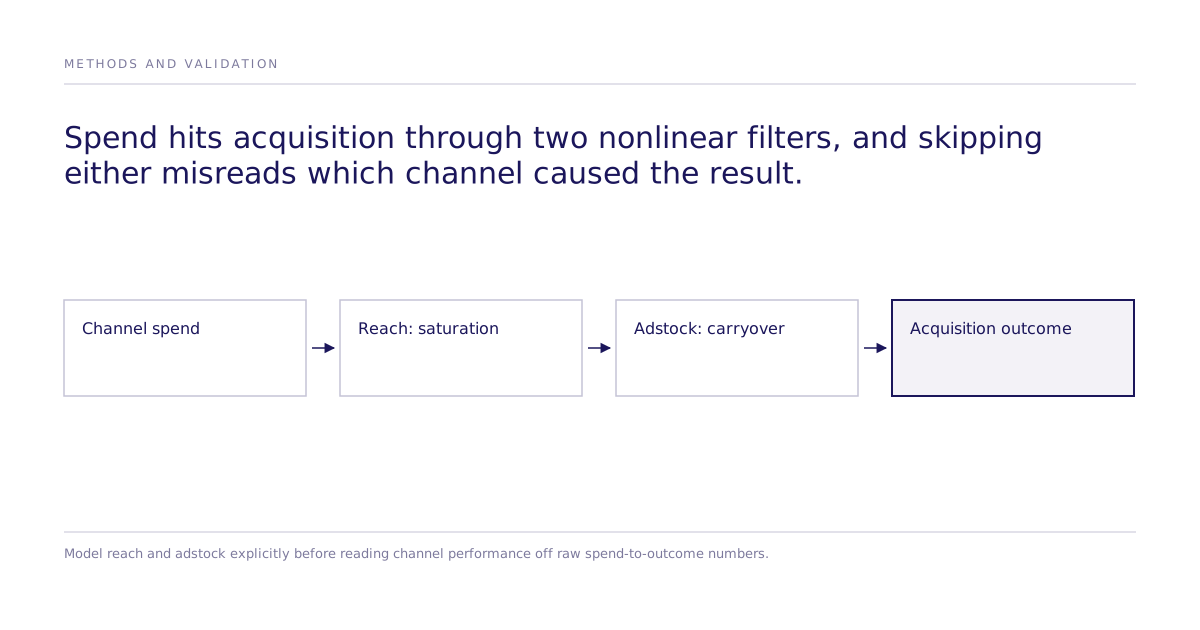
The reach function models saturation. The first dollars spent on a channel tend to produce the largest marginal gain in acquisitions. Additional spend on the same channel runs into diminishing returns as the audience becomes saturated with the message. A channel with room left on its reach curve and a channel near its ceiling can show similar week-over-week acquisition numbers, even though one has far more budget headroom than the other.
The adstock function models carryover. A channel's effect on acquisition does not end the moment spend stops. Some channels decay within days; others carry an effect for weeks. A channel that looks weak in a short attribution window can still be earning acquisitions from spend several weeks earlier. The adstock function recovers that long-tail effect from the data.
Cutting a channel that is actually mid-saturation, or one whose adstock decay hasn't finished, wastes the reallocated budget for a full cycle before the attribution error becomes visible in results.
What does the Bayesian layer add over a standard MMM?
A standard MMM fits reach and adstock parameters from historical data alone. The Bayesian version adds three properties that matter for a team making a budget decision:
- Prior knowledge from experiments and expert judgment can enter the model formally. A marketing manager's accumulated intuition about a channel, or the result of a completed lift or incrementality test, becomes a prior distribution rather than a fact the model has to rediscover from scratch in the current data.
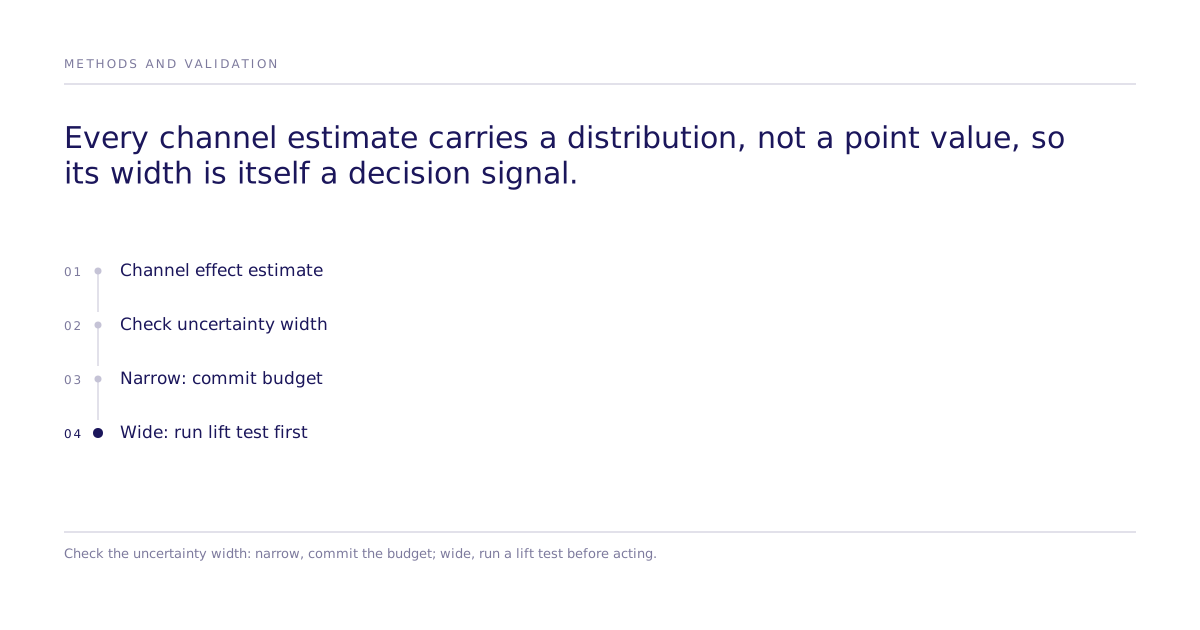
- Uncertainty propagates coherently through the nonlinear saturation and adstock transforms into ROI and optimal-allocation estimates, and priors act as regularization under the severe collinearity typical of channel spend data. A channel estimated with wide uncertainty is a signal to run a targeted lift test before committing more budget to it, not a number to treat as settled.
- The model updates as new spend and outcome data arrive, sharpening the saturation and carryover estimates for a channel within the period the model was fit on. Letting those estimates drift as market conditions change requires an explicit time-varying-coefficient or state-space specification, not just posterior updating.
Where fitting a Bayesian MMM gets hard in practice
Naming a failure mode before a team hits it is what makes the method usable. Building a Bayesian MMM is conceptually simple and operationally demanding. The practical stumbling points are consistent across implementations:
- Likelihood choice. Customer-count data can be modeled with a Poisson, negative binomial, normal, or longer-tailed distribution such as Student's t, and the choice changes how the model treats outliers and overdispersion.
- Prior specification. State-of-the-art models can carry hundreds of parameters across regression coefficients and reach/adstock shape parameters. Weak or poorly chosen priors are a common source of convergence failure.
- Reach and adstock parameterization. The functional form chosen for each affects how interpretable the resulting curve is and how directly it can inform a spend decision.
- Model comparison. Dozens of candidate MMM variants may need evaluation during development.
- MCMC convergence. Correlated chains, sampling divergences, and over-specified models can all produce a model that looks fit but has not actually converged. That failure mode is invisible without checking chain diagnostics directly.
None of these are unique to marketing. They are the standard costs of fitting a hierarchical Bayesian model with a large parameter count, and a team evaluating whether to build or buy MMM capability should budget for them.
Where pre-spend causal testing fits before an MMM does
MMM is retrospective: it explains what already happened to a channel's spend and outcomes. It cannot tell a team what would happen with an untested message or creative, or with a budget split outside the spend range it was fit on.
Subconscious's causal experimentation runs a randomized, discrete-choice-style test of a specific channel, message, or budget-allocation action before a team commits spend to it, producing a directional causal comparison with uncertainty language where the study design supports it. That is a complementary step upstream of MMM, not a substitute for it: Subconscious does not build or replace a Bayesian MMM, does not fit reach or adstock curves, and does not run MCMC inference. Where the decision depends on more than a directional read, a team can move from a simulated test to real-human validation of the same action without changing the causal question being asked.
What limitations should you keep in view?
Publishing where a model breaks is what lets a buyer check its number against reality. An MMM, Bayesian or otherwise, is an observational regression: its causal interpretation depends on no unobserved confounding and exogenous spend, assumptions routinely violated when budgets are set in anticipation of demand (seasonality, budget-follows-sales, competitive response). It only measures what happened in the spend and outcome data it was fit on, and its uncertainty estimates are only as trustworthy as its priors and convergence diagnostics. Pre-spend causal testing narrows a different kind of uncertainty: which of several untried actions is worth taking.
For a related discussion of causal versus predictive modeling, see how Subconscious approaches causal action testing and published case studies.