How CPG Teams Test a Price Increase Before a Shelf Reset
On this page
A revenue-growth or brand lead preparing for a shelf reset needs to evaluate a proposed SKU price, pack size, and competitive set. Scanner and household-panel records can inform demand models; a randomized choice study can test specified offers beyond observed prices. Neither route automatically establishes actual shelf sales at the new price. Choose a combined evidence plan for the retailer decision.
- Review the historical data's coverage, price support, promotions, availability, and identification before using its elasticity estimates.
- A demand system can estimate own- and cross-price relationships. Confounding and extrapolation need assessment rather than an assumption that scanner models are unusable.
- Hypothetical choice tasks can also overstate willingness to pay; a structured choice format does not remove hypothetical bias.
- Specify complete offers, the anticipated competitive set, status quo, and no-purchase option where relevant. Random assignment identifies the tested contrast on the recorded response under design assumptions.
- Report tested price support and uncertainty. Modeled preference shares need additional inputs and validation before they become a category-revenue claim.
What decision does a CPG team need to test before a shelf reset?
Record the actual line-review deadline and alternatives. For example, a hypothetical team might compare holding price, increasing price, or changing pack size before a reset scheduled in eight weeks. That calendar is an assumption, not a standard retailer window. Estimate margin, volume, distribution, and operational consequences for each alternative; they can create asymmetric risks.
What can scanner history contribute?
Scanner records show prices, transactions, and the channels they cover. A suitable model can use them to estimate demand relationships and predict scenarios, subject to identification and extrapolation assumptions. Display, feature, seasonality, stockouts, and endogenous pricing may influence the estimate. Investigate those factors instead of assuming every estimate combines price and promotion irretrievably.
What does data-source sensitivity mean?
Luke, Tonsor, and Schroeder's 2026 meat-demand paper compares Rotterdam demand systems using public and scanner data for 2009–2018. Elasticity magnitudes and classifications differ, but all compensated own-price estimates are negative. The paper estimates cross-price effects jointly. Differences in product and market coverage limit interpretation; the study does not establish that scanner elasticity reverses own-price signs or cannot answer a new-price question.
Hypothetical price responses have a separate limit
Schmidt and Bijmolt's 2020 meta-analysis covers 77 studies in 47 papers and reports average hypothetical WTP overstatement of 21%. Indirect methods overestimated more than direct methods on average. This is an aggregate across heterogeneous settings, not a method-specific adjustment for Gabor–Granger or Van Westendorp, and not evidence that DCEs avoid the bias. Use matched validation or appropriate real-stakes evidence; do not subtract 21% from every result.
What does a randomized shelf-reset price experiment look like?
Define current and proposed complete offers, competitor facts with source dates, pack sizes, budget and availability context, and the no-purchase option. Design assignment to identify the intended contrast: if price and pack size change together, the estimate concerns that combined offer. Specify model or human coverage, task burden, estimator, analysis, and decision threshold before fielding. Multinomial and mixed logit have different substitution assumptions; an estimator cannot create identification absent from the design.
Conventional approach and randomized experiment, side by side
| Historical demand model | Randomized choice study | |
|---|---|---|
| Price support | Observed prices; prediction beyond them requires assumptions | Assigned tested prices; extrapolation remains model-dependent |
| Cross-price effects | Can be estimated in joint demand systems | Can be modeled if alternatives and design support substitution analysis |
| Identification risk | Endogeneity, promotions, coverage, and specification | Assignment/design problems, response measurement, and population or model mismatch |
| Hypothetical bias | Observed transactions avoid stated-WTP elicitation; added surveys may not | Human stated or generated choice remains hypothetical unless real stakes apply |
| Output | Quantity and substitution estimates under the demand model | Choice contrasts or modeled shares under the study assumptions |
| Useful role | Baseline, calibration, and supported demand scenarios | Testing specified offer contrasts with independent transfer evidence |
What does the retailer actually want to see at the line review?
For a category-value scenario, specify incidence, buying occasions, quantity, outside options, prices, and distribution or availability assumptions. A forced single-SKU choice supplies no direct evidence of category dollars. Calibrate any conversion from choice shares to quantity using independent records and test against untouched outcomes. Present assumptions, sensitivity, and conditional intervals alongside the retailer-facing estimate.
How much can you trust a randomized price experiment?
The July 2026 causal fidelity working paper reports mean estimated choice-parameter rank correlation of 0.73 across 43 design-filtered studies and 0.55 across roughly 300 replications. These aggregate ranks do not validate retail price elasticity, absolute quantity, or revenue for this category. Per-study replication data are not public; the public evidence record is aggregate context. Independent new-task evidence is needed to assess training exposure and market transfer.
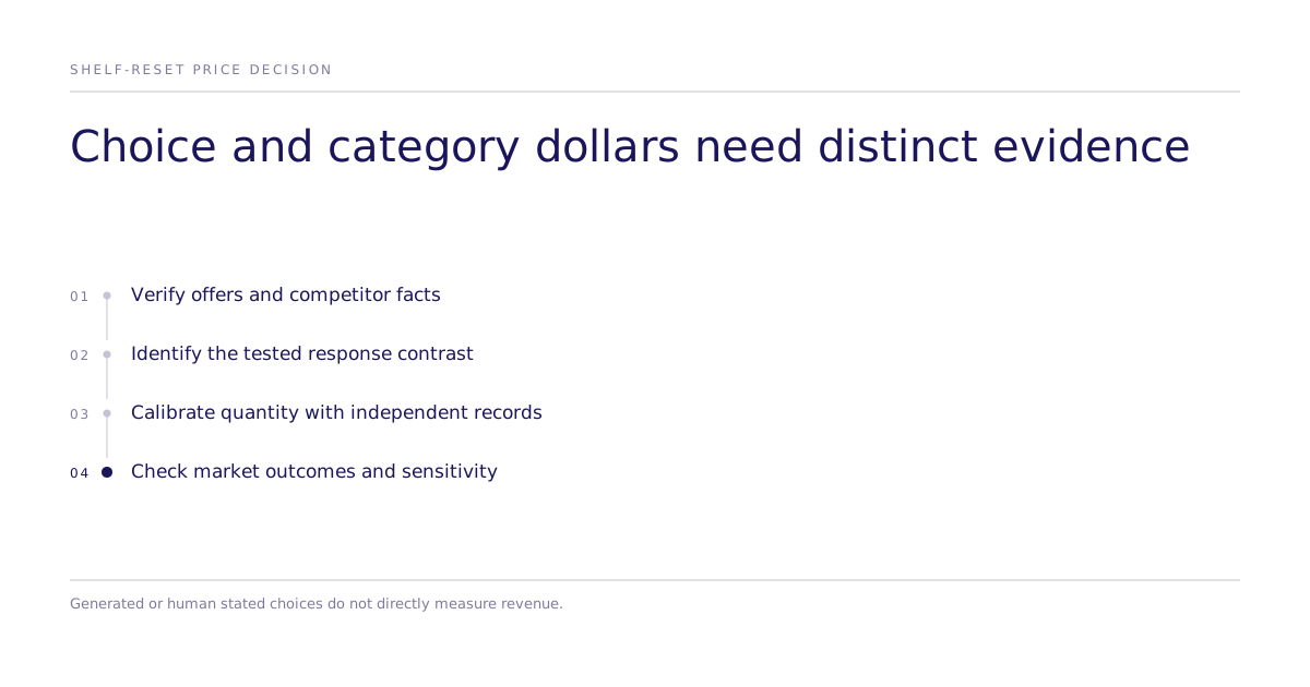
Gather current and proposed SKUs, prices, pack sizes, competitor-source dates, and the actual line-review deadline. Define whether the unknown is choice, quantity, margin, or category dollars. Discuss a study scope that combines available records with a suitable comparison and independent validation, retaining baseline and borderline alternatives.