Bayesian A/B Testing at Scale: Why Millions of Observations Slow MCMC Down
A head of experimentation with a large A/B dataset needs posterior estimates that finish in time to inform the decision. Observation-level likelihood evaluation can dominate MCMC cost, but a million rows is not a universal failure threshold. The likelihood, parameterization, hardware and sampler all matter.
What did the histogram benchmark show?
Ben Vincent’s PyMC Labs benchmark, February 12, 2026, uses normally distributed continuous outcomes in discrete test groups. Its histogram approximation weights each bin-center likelihood by its count, with 500 bins. On an iMac with an 8-core Intel i9 and 40 GB RAM, the reported results were:
| Setting | Reported time |
|---|---|
| 100 million observations, binned | 22 seconds sampling; about 30 including compilation |
| 500,000 observations, unbinned without indexing | About 75 seconds |
| 500,000 observations, binned | About 13 seconds |
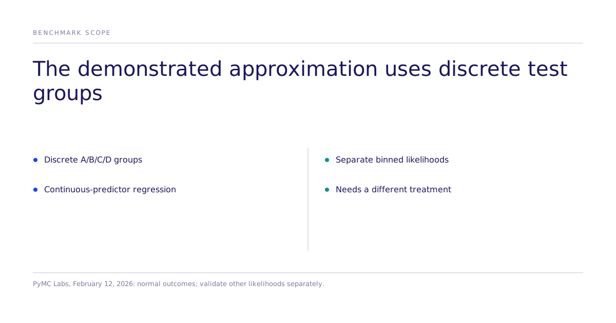
The post compares estimated uplifts across simulated datasets. These timings describe that author’s model and machine, not a general performance guarantee. The implementation supports multiple discrete groups; the post does not extend it to continuous-predictor regression.
What does the evaluation ratio measure?
For a single likelihood vector, 1,000,000 rows divided by 500 bins gives 2,000 times fewer evaluated locations per likelihood calculation. Count each group’s bins when comparing a multi-group model. This is a likelihood-evaluation reduction, not a runtime speedup. Compilation, gradients, sampler trajectories and diagnostics also cost time. Constructing the histogram still requires reading the original data.
How should a team validate the approximation?
- Compare posterior contrasts and decision probabilities against an unbinned fit on a manageable dataset.
- Increase bin resolution and check whether the decision changes, including sensitivity in the tails.
- Check convergence and effective sample size rather than timing alone.
- Choose a likelihood appropriate to the outcome. Counts, skewed values and heavy tails need suitable models.
Binning changes the data representation and introduces approximation error. For some likelihoods, exact sufficient statistics can reduce cost without that approximation. Evaluate the existing model before choosing a compression method.
What this means for the underlying decision
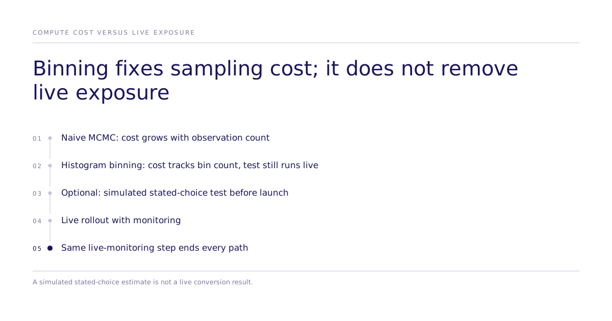
A speed fix and a live-exposure problem are separate claims. Binning solves the "MCMC compute grows with observation count" problem for a team willing to build and maintain that engineering. It does not solve a different, earlier problem: even a binned sampler still means the test may need to run against millions of real users to resolve small effects. Use a prespecified monitoring and stopping policy, practical loss thresholds and exposure limits; Bayesian inference alone does not define a safe rollout policy.
A separate screening study can run controlled experiments on a simulated population and estimate effects on modeled stated choices, with confidence intervals describing sampling variability within that simulation, before a change reaches a real customer. The assigned contrast is identified inside the configured model; human or live transfer requires matched evidence. A stated-choice estimate is not a live conversion result, and external validity to the real-customer population is a separate assumption. The July 2026 causal fidelity working paper, which is not peer reviewed, reports a mean Spearman rank correlation of 0.73 on estimated choice parameters across the 43 studies that passed its design filters, and 0.55 across roughly 300 replications. Those figures do not predict the result of a particular new test. Specify the comparator and endpoint in the study design.
Limitations
It is an engineering pattern for scaling a live pipeline. A simulated test run first does not remove the need to monitor a live rollout at scale once the change ships. The two are complementary steps in the same pipeline, not substitutes for each other.
Further reading
Other large-N approaches approximate the likelihood by subsampling rather than binning, including "Light and Widely Applicable MCMC: Approximate Bayesian Inference for Large Datasets" and "Informed Sub-Sampling MCMC: Approximate Bayesian Inference for Large Datasets". They are related methods, not the binning technique benchmarked above. The open-source PyMC library remains a common tool for building these models.
See the published evidence and its limits on the research page. To scope a specific test, book a decision review.