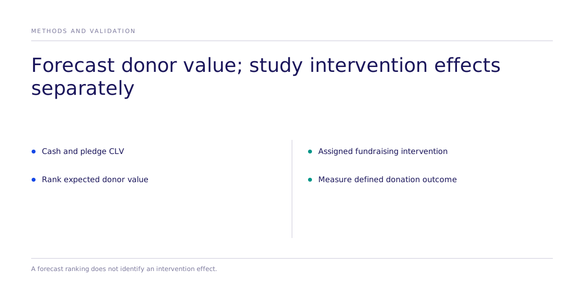
A Donor Value Forecast Does Not Identify Which Fundraising Action Works
Annika Denninger and Abdulhamed Chribati describe an independently developed donor-value MVP for an anonymous children's rights NGO in their personal-capacity PyMC Labs community report, dated April 17, 2026. This is their implementation report, not a Subconscious client case. Its forecasting methods help rank expected donor value; the report does not establish which fundraising intervention increases it.
The decision this model was built to inform
The NGO's fundraising and marketing teams needed to compare donor value, at the individual and segment level, to allocate budget toward expected long-term impact rather than short-term donation revenue. They wanted the resulting lifetime-value number to work as a core KPI: a common yardstick for judging acquisition channels and reading A/B test results.
That is a forecasting problem. Predicting a number and knowing what changes it are different questions, and the second one is where a budget decision actually lives.
What are the two donor types?
The team's data covered two overlapping donor behaviors: committed recurring giving ("pledge donors") and flexible, ad hoc contributions ("cash donors"). A single supporter could show both patterns over time. Most records started in 2018, with a subset of pledge histories going back to the 1990s. The team set 2024-01-01 as the train/test split, holding out roughly two years for out-of-sample testing.
They built one model per behavior:
- Cash pillar. A beta-geometric/negative binomial (BG/NBD) model forecast donation frequency, following the framework Fader, Hardie, and Lee proposed as an alternative to the Pareto/NBD model in Probability Models for Customer-Base Analysis. A Gamma-Gamma model estimated each donor's expected average cash donation amount. Cash CLV is the product of the two.
- Pledge pillar. A Shifted Beta-Geometric survival model, building on Fader and Hardie's approach to projecting customer retention in a discrete-time contractual setting, estimated donor survival curves. Multiplying survival probability by the most recent monthly pledge amount and summing over time produced pledge CLV.
Both pillars applied a 2% annual discount rate to account for currency devaluation, kept configurable rather than fixed. The team capped the forecast horizon at 10 years, judging that their observation window could not support reliable inference beyond that range given their donor base's loyalty patterns. Total donor-level value is cash CLV plus pledge CLV.
The authors recommend checking correlation between donation frequency and amount against a 0.3 rule of thumb when assessing the Gamma-Gamma independence assumption. Low correlation alone does not establish independence.
Why MAP replaced MCMC at this scale
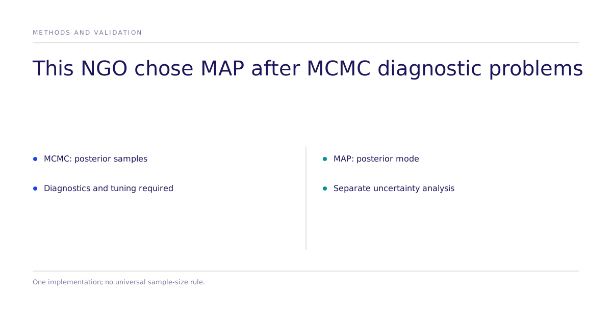
PyMC, the open-source probabilistic programming library underneath this work, supports several fitting methods. The team started with MCMC (Markov chain Monte Carlo) sampling, which approximates posterior distributions with samples rather than returning only a point estimate, useful because it lets a team assess uncertainty directly rather than assuming it away.
In this implementation, at their scale, more than a million data points, that advantage came with a cost. Sampling was compute-intensive, tuning draws, chains, and target acceptance rate took sustained iteration, and the team hit convergence and autocorrelation problems even after switching samplers. They eventually downsampled the data to keep MCMC runtime feasible.
They moved to MAP (Maximum a Posteriori) estimation instead: point estimates from an optimization over the posterior density rather than a full sampling process. For this implementation, MAP ran with less tuning overhead and avoided the convergence headaches, at the cost of losing built-in uncertainty quantification. MAP is still Bayesian: priors regularize the fit, but the team had to reason about uncertainty separately from the estimate itself.
MCMC is not generally wrong for large datasets. Runtime depends on model geometry, parameter count, available sufficient statistics, hardware and diagnostics. Posterior uncertainty can matter at any sample size. Choose an inference method against the decision and acceptable approximation error, rather than a universal data-size threshold.
What the model still leaves open
A CLV forecast can rank donors and segments by predicted value. It does not, by itself, identify whether a different ask amount, retention message or acquisition channel would increase donations. A high-value segment might be valuable regardless of the intervention.
To estimate an intervention's effect, define an outcome and comparison. For a retention message, randomly assign eligible donors to the new message or current practice, track donations and costs over a specified window, and analyze assignment rather than only message opens. A longer-term CLV outcome adds model assumptions to the measured short-term response.
A simulated choice task can screen described messages or offers, but its outcome is modeled stated choice within the configured population. A human choice task also measures stated choice; transfer to donation behavior requires matched evidence. The methods hub and research evidence help distinguish design from validation.
What are this model's limitations?
The NGO's own team flagged two open gaps in their model: it is revenue-driven and does not yet account for cost, and it does not model donors moving between cash and pledge behavior over time.
Review the revenue definition, handling of donor costs and movement between giving modes before using the score to allocate resources. The correlation check is a diagnostic, not proof of independence. Compare predictions with held-out outcomes by segment and donor tenure, and inspect sensitivity to the discount rate and forecast horizon.
Where does this fit in a budget cycle?
Use the CLV model to prioritize investigation. Use an intervention study to estimate what changes donations, and include costs when comparing actions. Forecast quality and intervention evidence answer different budget questions.