Hierarchical Bayesian Latent-Trait Estimation, Explained
A number published without its limits reads as marketing. Trusting a model's output for a pricing or positioning decision means trusting how it handles uncertainty. A single point estimate hides whether the underlying data supported the conclusion, and that gap only surfaces after the decision ships.
The estimation problem in plain terms
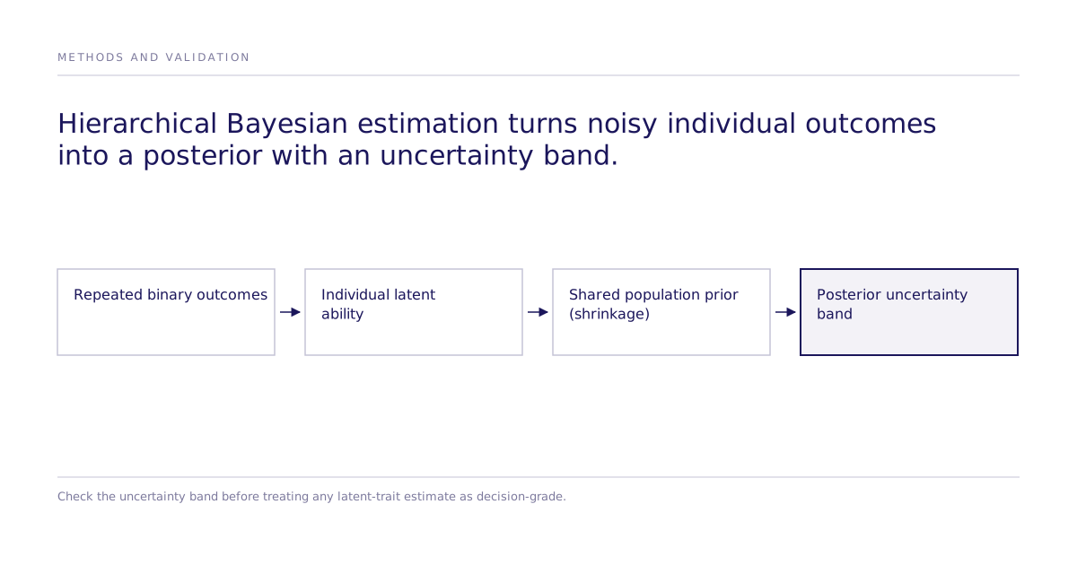
Austin Rochford’s NBA foul-call example, republished by PyMC Labs, models repeated interactions between the player committing a foul and the player fouled. Its role-specific latent traits describe foul-call tendencies in that dataset, not a general measure of individual ability. In the basic educational Rasch model, P(correct) = logistic(ability - item difficulty); fixing the population center or an anchor item identifies the scale.
Item Response Theory (IRT), and its simplest form the Rasch model, is a statistical framework built for this measurement problem: separating an individual's underlying trait from the noise in any single observation. It comes from educational and psychological measurement, estimating a test-taker's ability from a pattern of right and wrong answers rather than one score. Item Response Theory (Columbia University Mailman School of Public Health) frames it as modeling the probability of a response as a function of latent trait and item difficulty, not as a raw tally.
Why does hierarchy matter?
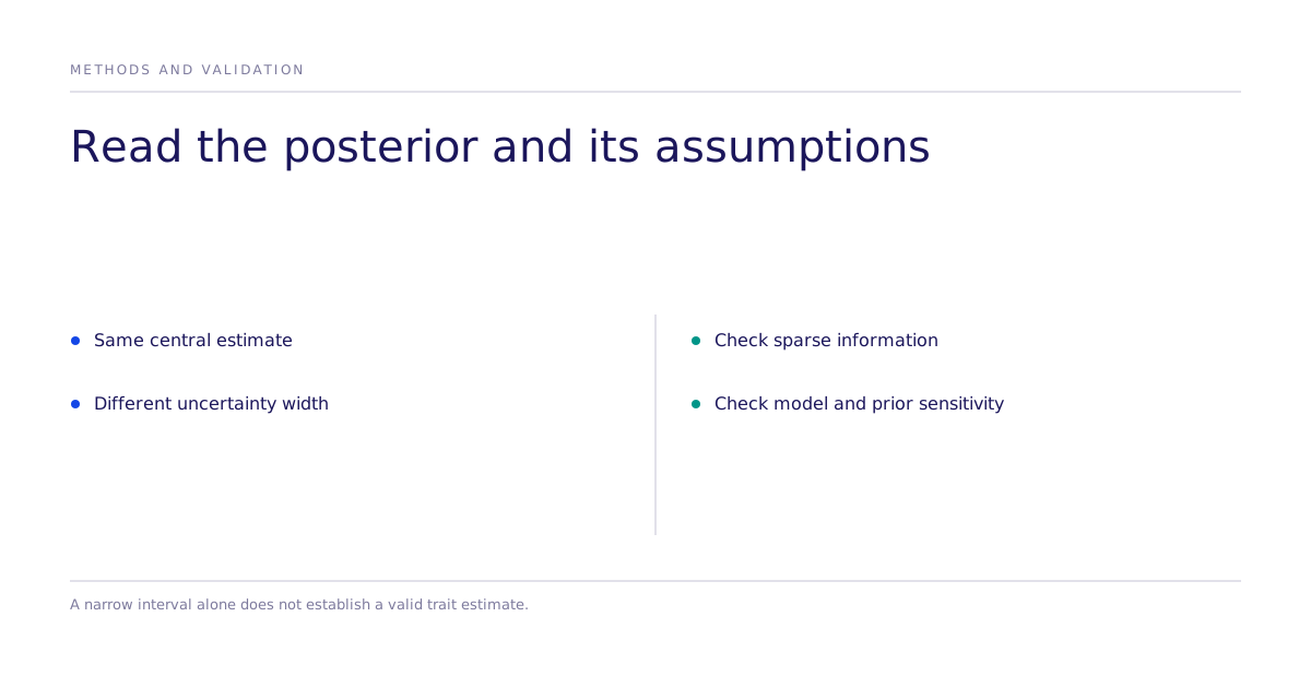
Hierarchical estimation can stabilize sparse individual estimates by partially pooling exchangeable individuals through a population model. The amount of pooling depends on sample information and the prior. Check prior sensitivity, posterior predictive fit, identification and whether the measurement model remains comparable across roles or groups before treating a score as a durable trait. A narrower interval alone does not prove that the latent construct is valid.
The result is not one number per individual. It is a posterior distribution: a full range of plausible values with a credible interval, rather than a single guess presented as fact.
Reading the posterior, not just the point estimate
Compare each central estimate with its uncertainty interval and the observations supporting it. Two individuals can show the same average estimate while one has a narrow, well-supported interval and the other has a wide one built on thin data. Collapsing both to a single ranking number destroys that distinction.
Reporting uncertainty is useful across inference methods, but their intervals have different meanings. Bayesian estimation produces posterior distributions and credible intervals. Likelihood-based choice estimation uses a sampling procedure for confidence intervals. Neither supplies causal identification by itself: that depends on the assignment design and its assumptions. For a Subconscious study, ask which estimator and uncertainty procedure were used and which human comparison supports the result; see the public working paper and evidence record.
What does this example establish?
The worked example above is a sports-analytics case study built to illustrate one estimation technique. It does not establish that any specific accuracy figure, ranking, or performance claim from that domain transfers to a marketing or consumer-behavior setting. What transfers is the estimation discipline: hierarchical priors, individual-level latent parameters, and a posterior interval instead of a bare score.
The buyer question this answers
For a decision based on a latent trait, ask what the parameter measures, how its scale is anchored, what evidence supports exchangeability and how sensitive the conclusion is to the prior. Then inspect uncertainty and predictive checks. Hierarchical Bayes is one possible analysis method; it does not establish which estimator a product uses. Scope the modeling decision around those checks.