Hierarchical Bayesian Models for Customer Lifetime Value Across Cohorts
A marketing analytics team comparing customer cohorts must decide whether to fit separate transaction models, one global model or a hierarchy that partially shares information. Small cohorts make that choice consequential. Forecast contribution-margin CLV with uncertainty, then combine it with acquisition cost and measured incremental response before allocating budget: a high predicted lifetime value alone does not show which cohort benefits most from additional spending.
Why cohort-by-cohort models break down
Probabilistic transaction models such as BG/NBD (Beta-Geometric / Negative Binomial Distribution) estimate purchase frequency and customer dropout from transaction history; BG/NBD alone has no monetary component, so a full CLV figure requires pairing it with a spend model such as gamma-gamma and a discount rate. A common workaround for seasonal or cohort-level differences is to fit one BG/NBD model per acquisition month.
This unpooled approach carries three costs:
- Model proliferation. A company running in 10 markets with two years of monthly cohorts needs 240 separate models.
- Cold start. A newly acquired cohort has too little transaction history to produce a stable estimate on its own.
- Arbitrary boundaries. Treating a customer acquired May 31 as fundamentally different from one acquired June 1 is rarely justified by the underlying behavior.
A single global model avoids all three problems, but it erases real differences between cohorts: a new, high-intent cohort gets the same parameters as an old, lapsed one.
What is partial pooling in a hierarchical Bayesian model?
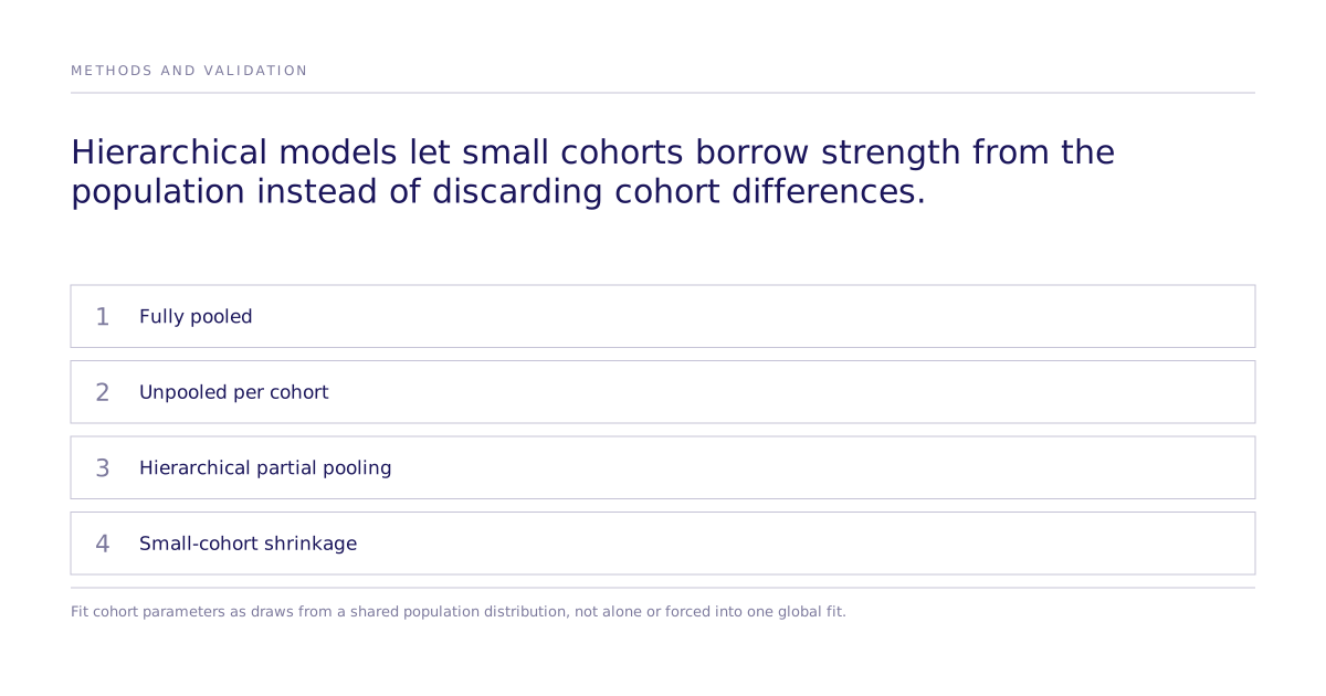
A hierarchical Bayesian model treats each cohort's BG/NBD parameters as draws from a shared population-level distribution, rather than fitting each cohort in isolation or forcing every cohort to share one set of parameters. This partial pooling lets small cohorts borrow statistical strength from the population while keeping their own signal.
Fader, Hardie and Lee provide the foundational BG/NBD model; Abe studies a hierarchical Bayes Pareto/NBD extension. The four-group BG/NBD comparison below is a separate PyMC Labs worked example by Juan Orduz. These sources should not be treated as the same model or experiment.
What the CDNOW example shows
The CDNOW customers were split into four acquisition-cohort groups of uneven size: 1065, 815, 353, and 124 customers. The fourth group is a realistic stand-in for a small or newly acquired cohort.
Fitting an independent BG/NBD model to each group produced four latent parameters, r, α (alpha), a, and b, governing purchase rate and dropout probability. For the two smallest groups, the a and b estimates showed high volatility and wide credible intervals: exactly the instability that makes an unpooled model risky to act on.
In the PyMC Labs example, hierarchical estimates pool information across the four groups and reduce uncertainty for some small-group parameters. That fitted-model comparison does not by itself establish better future CLV forecasts. Compare held-out transaction counts, spend, interval calibration and prior sensitivity before using the model for a budget decision.
Comparing the three approaches
| Approach | What it assumes | Failure mode |
|---|---|---|
| Fully pooled (one global model) | All cohorts share identical parameters | Erases real cohort differences |
| Unpooled (one model per cohort) | Cohorts are fully independent | Unstable estimates for small or new cohorts |
| Hierarchical (partial pooling) | Cohort parameters are draws from a shared population distribution | Over-shrinkage: if a small cohort is genuinely extreme, its estimate is biased toward the population mean and its narrowed interval can undercover |
Where does this reasoning apply beyond CLV?
Partial pooling is also an option for sparse survey or choice segments when the grouping and exchangeability assumptions are justified. It can reduce estimation variance while introducing bias for genuinely unusual segments. Ask which procedure a configured study uses and inspect validation for the decision; current research provides the public evidence context.
What are the limitations of this approach?
This is a modeling technique for observed transaction histories, not a description of a Subconscious product feature. This article's public sources do not document a Subconscious hierarchical BG/NBD validation or customer result; request evidence for the proposed modeling engagement. The technique also assumes cohort membership is a meaningful grouping variable; a poorly justified grouping can undermine the pooling assumptions, even when the fitted intervals look narrow.
Extending this approach with time-varying global parameters for seasonality, covariates for acquisition channel or demographics, or additional levels of hierarchy for multi-market data is straightforward, but it adds inference complexity that should be weighed against the size of the decision it is informing.
Next step
For a budget example, compare cohorts using predicted discounted contribution margin, acquisition cost and the incremental retention or acquisition effect measured in a pilot. Propagate uncertainty in each input. If the intervention response is unknown, use the CLV forecast to frame a bounded pilot rather than declaring a budget winner. See applied study examples or scope that pilot.