Likelihood Approximations Through Neural Networks: A Validation Checklist Before You Trust the Output
A behavioral model that reports a choice probability or a causal effect is only as trustworthy as the likelihood behind it. When that likelihood has no closed form, a team has to decide whether to accept the model's output on faith or check it against the simulator that generated its training data first.
This walkthrough draws on the PyMC Labs tutorial (March 31, 2023), written by Vieira, Fengler, Omar and Xu. It explains simulator checks for an approximate likelihood and the additional validation needed before its posterior informs a decision.
Why some models have no likelihood to evaluate
Standard Bayesian inference needs a likelihood function that scores how probable the observed data are under a given set of parameters. Many models used to analyze reaction times and choices don't have one in closed form.
The example model is a Drift Diffusion Model (DDM), a common framework for joint reaction-time-and-choice data. A DDM describes a decision as a random walk: evidence accumulates at a drift rate toward one of two boundaries, and whichever boundary is crossed first determines both the choice and the reaction time. The standard DDM has a known analytical likelihood, but realistic variants do not. One example is a variant where the decision boundary narrows as a deadline approaches. Those variants remain easy to simulate; you can generate synthetic trials from them in a few lines of code. They're just hard to score directly.
That gap between "easy to simulate" and "hard to score" is what simulation-based inference (SBI) is built to close.
What is the three-step pipeline for simulation-based inference?
Simulation-based inference replaces the missing analytical likelihood with a learned approximation, trained entirely on simulated data:
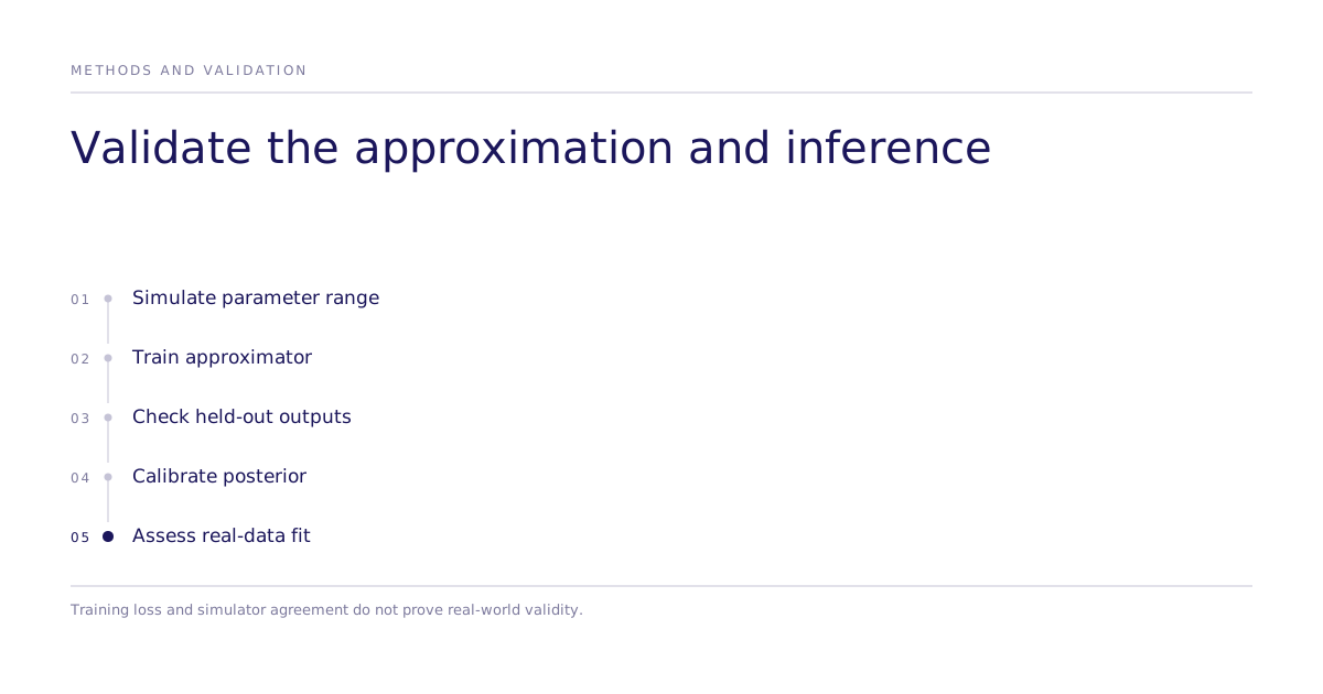
\text{simulate} \rightarrow \text{train an approximator} \rightarrow \text{validate against the simulator}- Simulate. Generate trials across many parameter settings. The tutorial first illustrates the simulator with 1000 trajectories at one setting, then separately generates training data across many parameter configurations.
- Train an approximator. Fit a neural network on the simulated data so it learns to score data the same way a true likelihood would. The source example trains two specialized networks, one scoring the reaction-time density for observed responses and one scoring how likely a response was withheld, and combined the pair spans the full likelihood.
- Validate against the simulator. Before the trained network goes anywhere near a real inference run, its output has to be checked against the simulator that generated its training data.
Step three is where most of the risk in this workflow lives, and the easiest step to skip under time pressure.
What does "validate against the simulator" actually mean?
Start with visual and numerical comparisons at held-out parameter values. Check density normalization, behavior near the edges of the training range, and approximation error where the posterior concentrates. Then use repeated simulated datasets for parameter recovery and posterior calibration, and check whether the simulator describes the real process. Agreement with the simulator cannot establish that last condition.
For the reaction-time network, that means plotting the network's predicted likelihood curve directly against a histogram of reaction times the simulator generated at the same parameter setting, for several settings across the plausible parameter range. For the choice-probability network, it means overlaying the network's predicted probability against the simulator's own observed choice frequencies. Both checks are described in Fengler et al.'s work on likelihood approximation networks for cognitive neuroscience, the peer-reviewed source for this class of approximation.
This is the checkpoint that separates "the network converged during training" from "the network's output means what I think it means." A network can report a low training loss and still produce a likelihood surface that diverges from the simulator in the regions of parameter space that matter for a specific dataset.
The broader case for this approach, using a trained approximator instead of an intractable likelihood and treating the approximator as something to validate rather than trust by default, is laid out in Cranmer, Brehmer, and Louppe's survey of simulation-based inference.
How is the validated network wired into a Bayesian model?
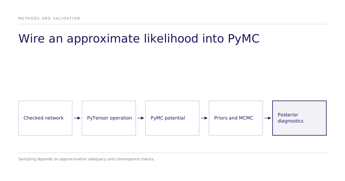
Once a network's output has been checked against the simulator, it can be dropped into a probabilistic model. In the source workflow, the trained networks are wrapped as custom PyTensor operations and injected into a PyMC model as potential functions, a mechanism for adding a custom log-likelihood term rather than using a built-in distribution. From there, standard Bayesian machinery applies: priors go on the model's parameters, and Markov chain Monte Carlo sampling produces a posterior distribution rather than a single point estimate.
The tutorial’s inference example uses 500 trials in each of two conditions; those counts describe the example data being fitted. Training uses a separate simulation dataset spanning many parameter settings. Its two networks train for 10 and 20 epochs. These are example settings, not validated sample-size or training recommendations for another model.
Recovering the true generating parameters from synthetic data, checking the posterior lands where you know the answer because you generated the data yourself, is the same closing step. It's a necessary check before the pipeline runs on data whose true answer is unknown, though recovering parameters from a single synthetic dataset doesn't by itself confirm the pipeline is correct across the board.
Where this discipline matters beyond one tutorial
The specific failure mode this validation step guards against is general: any model whose output feeds a business decision but whose fit was never checked against the simulator or dataset that generated it is a black box wearing a probability distribution. The number in the answer is real; whether it means what the reader thinks it means is not.
A buyer evaluating Subconscious research should ask which experimental design identifies the target effect, which estimator reports uncertainty, and which human comparison checks the intended outcome. A randomized design and an interval answer different questions from model calibration. The decision workflow should make each check inspectable.
Limitations
This is a methods walkthrough on likelihood-free Bayesian inference for drift diffusion models, built around open-source PyMC tooling. The public company sources linked here do not document deployment of this exact neural-network-likelihood workflow or DDM-specific tooling; confirm the intended implementation and deliverables for a particular engagement. The general lesson, approximate a missing likelihood and then validate that approximation against the simulator's own output before it informs a decision, is the part worth carrying forward regardless of which models or software a team uses.