Marketing Mix Modeling: A Complete Guide

Edited by Avi Yashchin, CEO and Co-Founder · August 19, 2026

Marketing mix modeling relates historical outcomes to transformed media inputs and other drivers. Adstock represents carryover; saturation represents diminishing returns. The resulting channel contributions depend on the model and causal assumptions. They do not automatically identify incremental sales.

What an MMM decomposes

MMM starts with a specified statistical decomposition:

Observed sales equal a base level, plus whatever lift gets attributed to TV, digital ads, promotions, and other factors.

The model assigns outcome variation to media inputs, controls, and residual variation. A basic linear regression treats effects as immediate; adstock and saturation allow more flexible response shapes.

Four interval checks: frequentist repeated-sampling coverage, uncertainty in fitted transforms, Bayesian conditional posterior probability, and sensitivity to priors. — Both approaches can report uncertainty; check its interpretation and propagate uncertainty in channel effects and transforms into allocation.

Why the basic equation isn't enough

Carryover and saturation differ by channel and campaign. A fitted model must support those differences from data or defensible prior information; TV and digital channels do not have universal decay patterns.

To reflect this, MMM adds two transforms before the regression step: adstock, which captures lag and carryover, and saturation, which models diminishing returns.

What is the adstock carryover effect?

An ad's effect doesn't land only in the week the money is spent. Some viewers act that week, some weeks later, some never. Adstock creates a transformed version of the spend variable that carries a fraction of each week's effect into the following weeks:

Adstock_t = Spend_t + \lambda \cdot Adstock_{t-1}

The current period's adstocked value is that period's spend plus a decayed fraction of the prior period's adstock, and so on backward. λ (lambda) sets the decay rate: a channel with a high λ retains more of its modeled effect across periods, while one with a low λ retains less. As a historical planning example, $1M spent on TV in week 1 with λ = 0.8 decays to $0.8M in week 2, $0.64M in week 3, and $0.51M in week 4.

What causes diminishing returns in marketing spend?

Even after adstock, more spend doesn't produce proportionally more sales. The first dollars reach the most responsive part of the audience; later dollars reach people who are harder to convince. Before that adstocked spend goes into the regression, MMM passes it through a saturation function, and a handful of function families show up repeatedly:

Logarithmic: f(x) = log(1 + x). Steep growth at low spend, flattening as spend rises.
Hill: f(x) = x^α / (x^α + θ^α). α controls how sharply the curve bends toward saturation; θ is the half-saturation point, the spend level where the channel delivers half its total modeled impact.
Tanh: f(x) = b * tanh(x / (b * c)). b sets the ceiling on impact the channel can deliver; c governs the curve's approach to that ceiling.
Logistic: f(x) = (1 - e^(-x)) / (1 + e^(-x)). For this unit-scale form, the half-saturation point is log(3); adding a scale parameter changes that point.

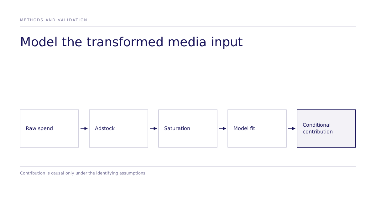
With both transforms in place, the flow runs: raw spend, then adstock (carryover), then saturation (diminishing returns), then regression. Each channel's estimated contribution is a coefficient applied to its saturated, adstocked spend; the base term is the model's residual level given the specified controls like price and trend, not an identified no-marketing counterfactual, and it can absorb brand equity built by prior marketing along with any omitted driver.

Control variables: what isn't marketing

Controls can help address confounding when selected under an explicit causal model. They do not guarantee identified lift: endogenous spend, omitted causes, and conditioning on mediators or colliders can distort estimates. Meridian’s causal guidance describes the assumptions; experiments can supply additional calibration evidence.

How do frequentist and Bayesian intervals differ?

Once the model's structure is set, its parameters (the channel coefficients and the adstock/saturation parameters) still have to be estimated from historical data. There are two common approaches.

The classic route is frequentist estimation: the nonlinear adstock and saturation parameters are fit by grid search or nonlinear least squares, and the channel coefficients are then estimated by ordinary least squares (OLS) regression conditional on those fixed transform parameters, producing a best-fit number for each coefficient along with a standard error and confidence interval. Those intervals come from repeated-sampling theory rather than a probability statement about the true effect, and are not posterior probabilities. Domain information can inform constraints, model specification or regularization, but those choices need justification and do not turn a confidence interval into a credible interval.

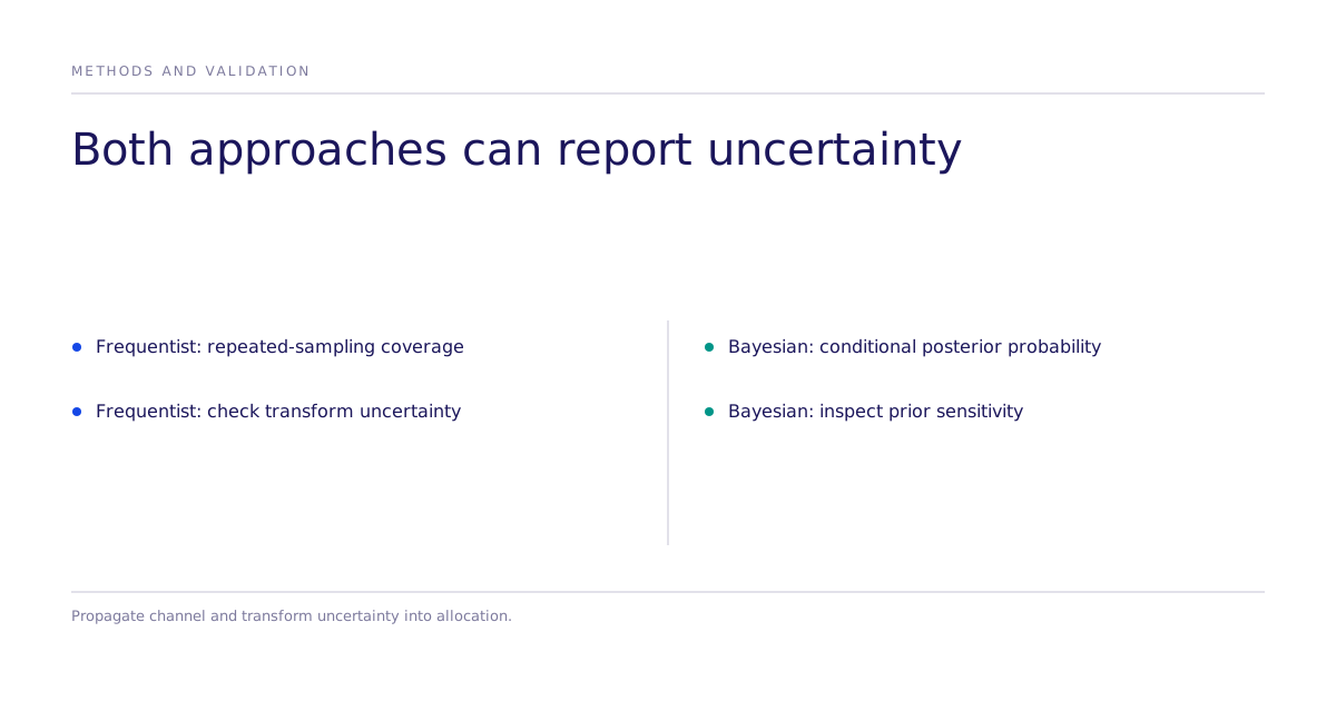
Both approaches can report point summaries and uncertainty. A frequentist confidence interval concerns coverage under repeated sampling; a Bayesian credible interval expresses posterior probability conditional on the model and prior. For budgeting, check whether uncertainty in adstock, saturation, and channel coefficients propagates jointly into the response and allocation. Conditioning on fixed transforms can understate uncertainty.

The same distinction matters when evaluating Subconscious experiments: ask which estimator produces the interval, what assumptions it conditions on, and which population and endpoint it describes.

What can't a marketing mix model do?

MMM needs enough independent variation to separate channel responses from seasonality and other drivers. The usable aggregation level depends on the available data and model, rather than a universal weekly or monthly rule. Historical fit alone does not establish causal returns or identify the contribution of an individual creative.

Lift experiments can calibrate an MMM when population, dates, channels, and outcomes align. A replication test needs predeclared agreement and failure criteria. The leaderboard reports research evidence; it does not guarantee agreement for a new operational result.

How does an MMM become a bounded budget recommendation?

For an illustrative weekly dataset, align spend, sales, prices, distribution, and seasonality to the same periods. Check that channel spend varies independently enough to estimate separate effects. Hold out later periods without using their outcomes during tuning; compare predictive error and calibration with simple baselines.

For a fixed budget, compare each channel’s marginal response over the spend range actually observed. Propagate parameter uncertainty and constrain minimum commitments, capacity, and maximum changes. If two allocations have overlapping uncertainty, present the tradeoff and run a targeted lift test. An optimizer extrapolating beyond supported spend levels can produce a precise but unsupported allocation.

Five boxes left to right: raw spend feeds an adstock transform carrying lagged effect forward, then a saturation transform that flattens at high spend, then regression, then each channel's contribution. — A channel's reported contribution reflects two transforms applied before regression, not the raw spend number itself.