When a Fixed CAC Assumption Misleads a Budget Reallocation
The decision this affects
A fixed channel-effectiveness parameter is one modeling option. Before using an MMM to set next quarter's budget, ask whether effectiveness is fixed or allowed to vary, which evidence identifies that variation and whether the proposed spend remains within support. A historical fit alone does not answer those questions.
How can a constant-CAC assumption affect allocation?
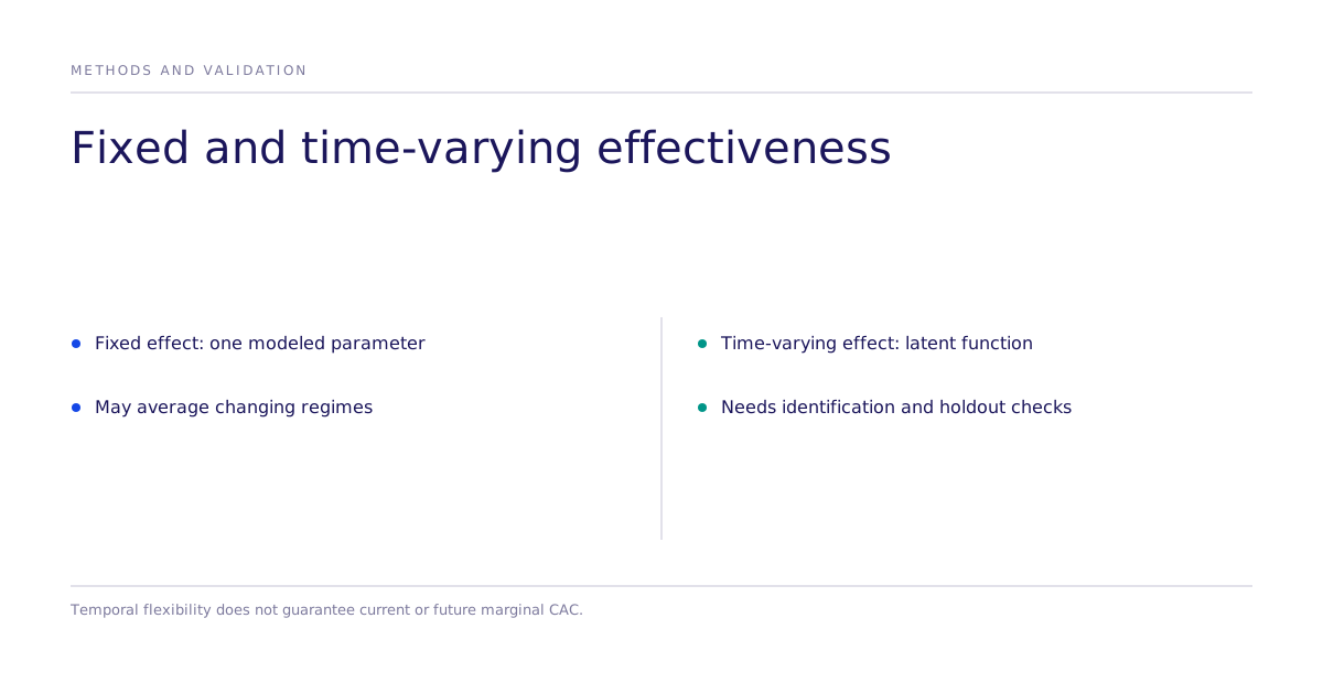
A media mix model with fixed channel effectiveness estimates one parameter across its training window. If the true response changes over that window, the fixed specification can misrepresent the response relevant to the next allocation. The direction and size of the error depend on spend, the response curve and the fitted baseline. Temporal holdouts, residual checks and relevant experimental evidence can expose problems before budget moves; a good headline fit alone cannot exclude them.
Audience behavior, auction dynamics, creative fatigue, platform policy changes and macro shocks can change channel performance. A fixed parameter cannot represent that variation directly, while a time-varying estimate still depends on how the model separates these influences. In the saturation example below, the efficiency parameter describes low-spend CAC; reallocating at current spend instead requires the marginal response and its uncertainty.
How does a time-varying model represent the same channel?
The fix does not require abandoning the interpretable model most teams already use. A standard saturation curve maps spend to acquired customers with two parameters: one sets the ceiling on how many customers a channel can produce at full saturation, and the other, the inverse of the curve's initial slope, represents the cost of acquiring a customer when spend is still low. Classically, that second parameter is treated as a fixed constant for the whole model.
The PyMC Labs effectiveness-over-time example illustrates latent time variation in a saturation parameter. That estimate must be separated from baseline demand, seasonality and correlated channel activity through model assumptions and relevant evidence.
How does the model infer effectiveness it never observes directly?
Because you only ever observe spend and customers acquired, the time-varying efficiency parameter has to be estimated, not read off. A Gaussian process is a standard way to do that: it puts a prior over smooth functions of time, encoding the assumption that channel effectiveness drifts gradually rather than jumping erratically day to day. Combined with the saturation curve, that lets the model produce a posterior estimate of gradual drift in efficiency; capturing seasonal patterns typically needs a periodic kernel, and abrupt shocks like a sudden shift in platform rules typically need a changepoint or shorter lengthscale, since a single smoothness prior trades off against representing both at once.
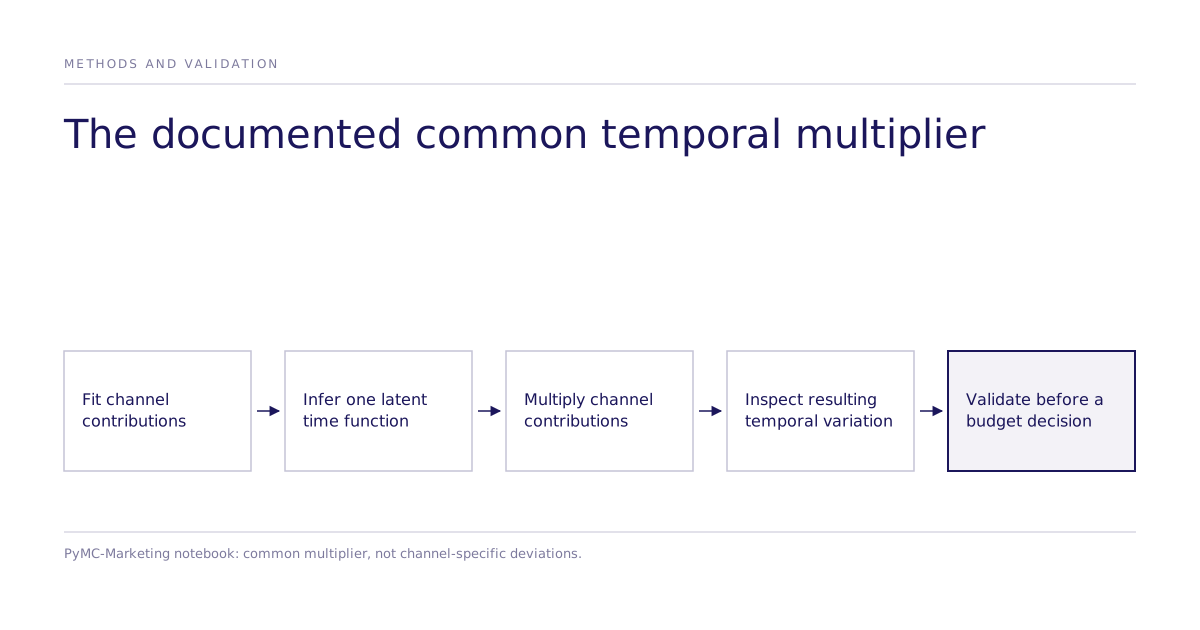
A different PyMC-Marketing time-varying-media notebook uses an HSGP temporal latent multiplier applied to channel contributions. In that implementation, the latent HSGP coefficients do not have a channel index: the time function is common to the channels. It does not demonstrate a shared market trend plus independent channel-specific deviations.
Where this connects to testing an action before you commit budget
This is a modeling example, rather than evidence of a Subconscious MMM feature. Time variation can improve a representation of historical effectiveness, but causal interpretation still needs identification assumptions. A randomized choice task answers a different question from operational channel allocation. See the methods and validation hub.
Review an applied case for its actual model, tested intervention, comparator and outcome. When planning a new allocation study, confirm the required evidence and deliverables.
What this technique does not tell you
A time-varying model does not guarantee that its latent function isolates genuine channel change or predicts an unsupported budget action. Check temporal holdouts, sensitivity, confounding and relevant experimental calibration before using the forecast.
The practical takeaway
Before reallocating, distinguish average CAC, marginal CAC at the proposed spend and uncertainty about future effectiveness. Compare fixed and time-varying specifications using relevant temporal holdouts and intervention evidence. Neither automatically supplies next quarter's marginal response.
---
[^1]: MMM with time-varying media baseline: PyMC-Marketing documentation, PyMC-Marketing (open source documentation).