GPU Sampling vs. CPU Sampling for Bayesian MCMC: When Is the Switch Worth It?
A data science team running MCMC-based causal inference in PyMC or Stan eventually hits the same question: move sampling to GPU, or stay on CPU? Getting it wrong either way costs. Accelerating a model that never needed it burns engineering hours nobody gets back. Staying on a CPU sampler past the point where GPU sampling would help stalls model iteration and delays whatever decision depends on the result.
What did the benchmark actually measure?
Martin Ingram of the PyMC Labs research team published one benchmark of this tradeoff on 22 December 2021 (PyMC Labs, "MCMC for Big Datasets: JAX and GPU Sampling with PyMC"). He fitted a hierarchical Bradley-Terry model, the standard pairwise-comparison model used for ranking competitors from win/loss records, to 160,420 professional tennis matches, on a Razer Blade laptop with an NVIDIA RTX 2070. The post links a reproduction repository, martiningram/mcmc_runtime_comparison. It compared standard PyMC, PyMC with a JAX backend on CPU, PyMC with JAX on GPU, and Stan, at dataset sizes ranging from a single recent year up to the full match history.
These are the original benchmark's figures, kept here as a planning example from that specific setup rather than a claim about current PyMC, Stan, or JAX performance:
| Sampling configuration | Runtime on the full 160,420-match dataset, in minutes |
|---|---|
| PyMC with JAX on GPU, vectorized | ~2.7 |
| PyMC with JAX on GPU, parallel chains | ~4.5 |
| PyMC with JAX on CPU, parallel chains | ~7.5 |
| Standard PyMC (CPU) | ~12 |
| Stan via cmdstanpy | ~20 |
On the table above, the 2.7-minute GPU run is about 2.8 times faster than the 7.5-minute JAX CPU run, 4.4 times faster than standard PyMC, and 7.4 times faster than Stan. The post summarizes a fourfold GPU advantage over its quickest CPU approach, which its table does not support against the JAX CPU run (about 2.8x). The 4x figure matches the comparison with standard PyMC. These ratios apply to this historical setup, not a general GPU guarantee. The benchmark also reported effective-sample-size-per-second gains of roughly 11x for the vectorized GPU method versus standard PyMC and Stan, meaning the GPU run produced more usable independent samples per second, not just a shorter runtime. Even without a GPU, running PyMC with a JAX backend on CPU alone delivered about 2.9x more effective samples per second than standard PyMC and Stan.
Where does the CPU-to-GPU crossover point sit?
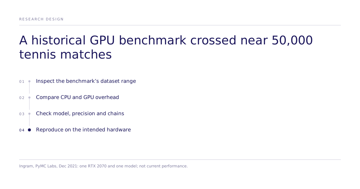
The benchmark's runtime curves were close to flat for GPU configurations across dataset sizes, while CPU runtime grew with data volume. That produced a crossover point: below roughly 50,000 tennis matches, GPU sampling ran behind CPU because of fixed per-run overhead; above it, GPU sampling won. For a team deciding where to spend engineering effort, that crossover point matters more than the headline 2.7-minute runtime, because it tells you whether your own dataset is even in the range where the investment pays off.
What doesn't generalize from this benchmark?
The setup that produced these numbers was narrow, which matters for anyone using the crossover point as a planning guide:
- One model class. The benchmark used a single relatively simple hierarchical model. More complex models, including ones with additional covariates or dense covariance structures, may see a different crossover point or a different relative ordering of methods.
- One consumer GPU. Testing ran on a single RTX 2070, not a data-center GPU or a multi-GPU cluster. Results on different hardware, or at larger scale, were not measured here.
- Dated software versions. The benchmark used PyMC v4, cmdstanpy v1.0.0, JAX v0.2.13, numpyro v0.8.0 and CUDA 10.1. Current releases can produce materially different timings for the same model and hardware.
- Unvalidated precision tradeoff. The post noted a theoretical 32x gap between the RTX 2070's rated double-precision throughput (233 GFLOPS) and single-precision throughput (7.465 TFLOPS), and said switching to float32 could give a further speedup but needs careful validation of numerical stability before adoption. Treat that figure as an open question, not a confirmed gain.
Before committing to GPU sampling
Check where a candidate dataset falls relative to the roughly 50,000-match range where this benchmark found GPU sampling starts to win, and treat that boundary as a reference for a similar model class, not a universal threshold. Then reproduce the comparison with the intended model, data, precision, chain configuration, and hardware before choosing a backend. For teams building causal research into decision infrastructure, the relevant question is whether the sampling design supports the decision without changing it. This historical benchmark does not establish current platform performance or imply that Subconscious uses the same stack.