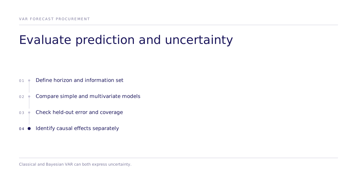
When Metrics Predict One Another: A Buyer's Guide to Vector Autoregression
An analytics leader forecasting several business metrics should ask whether
their histories improve prediction of one another. A vector autoregression
can model those cross-lag relationships. Compare its performance with simpler
forecasts on held-out periods before adding complexity. Predictive improvement
does not establish that intervening on one metric will change another.
What can't a single-equation forecast see?
A standard autoregressive forecast predicts one metric from its own history.
A univariate autoregression uses the metric's own past. It may be a useful
baseline even when other variables matter. Adding their histories is worthwhile
only if the resulting forecast improves under an appropriate evaluation.
y_t = a + b_1 y_{t-1} + b_2 y_{t-2} + \ldots + b_n y_{t-n} + \epsilonHere the left-hand side is the metric's value at the current time step, the
first term on the right is a baseline intercept, each following term weights
how much an earlier value of the same metric still matters, and the last
term is unexplained noise. Nothing in this equation lets a second metric
contribute at all.
How does vector autoregression model cross-lag prediction?
A vector autoregression (VAR) model replaces the single equation above with
one equation per metric, and each equation includes the recent history of
every other metric in the system:
y_t = a_y + b_{yy,1} y_{t-1} + b_{yy,2} y_{t-2} + b_{xy,1} x_{t-1} + b_{xy,2} x_{t-2} + \epsilon_yx_t = a_x + b_{yx,1} y_{t-1} + b_{yx,2} y_{t-2} + b_{xx,1} x_{t-1} + b_{xx,2} x_{t-2} + \epsilon_xSetting every cross-term to zero collapses the system back into two
independent, single-metric forecasts. Keeping them in is what lets the model
represent predictive relationships among the metrics. Cross-lag coefficients
do not identify intervention effects without additional causal assumptions.
For a business example, sales and inventory may each contain information
about future values of the other. Promotions, supply constraints, and seasonality
may also affect both. Define the forecast horizon, data available at prediction
time, lag order, transformations, and baseline before evaluating the model.
Check for instability or regime changes that weaken historical relationships.
What changes when the VAR is Bayesian?
Both classical and Bayesian VAR can quantify uncertainty. Statsmodels
documents classical forecast intervals under Gaussian assumptions
(VARResults.forecast_interval).
A Bayesian VAR combines an explicit likelihood with priors to estimate a posterior.
| Classical VAR | Bayesian VAR | |
|---|---|---|
| Coefficient uncertainty | Sampling-based estimates and intervals | Posterior distribution conditional on likelihood and priors |
| Forecast uncertainty | Forecast intervals under model assumptions | Posterior predictive distribution under model assumptions |
| Regularization | Can use frequentist penalties or constraints | Can use shrinkage or hierarchical priors |
| Buyer check | Held-out forecast error and interval coverage | Held-out forecast error, coverage, and prior sensitivity |
The PyMC example gallery
demonstrates simulated-data recovery, comparison with Statsmodels fits,
and hierarchical modeling. PyMC requires a specified model and checks;
writing equations alone does not guarantee useful Bayesian inference.
A technical example to inspect
PyMC Labs' Bayesian vector autoregression article
is the original source for this guide's modeling topic. Use its implementation
alongside the PyMC gallery to inspect how cross-lag terms enter the equations.
Ask for code, data revisions, prior choices, diagnostics, and held-out evaluation
for your own forecast. A coefficient near zero in one example does not establish
that the corresponding business relationship is absent in a new dataset.
For procurement, compare a univariate baseline, a multivariate model, and
any operational forecast at the same horizon with the same information set.
Evaluate error, interval coverage, decision cost, and robustness to regime changes.
How does this relate to decision experiments?
A forecast asks what may happen given a history and specified assumptions.
A decision experiment asks how a tested intervention changes a measured response.
Discuss a Subconscious study separately if the decision involves buyer choices;
confirm its audience, assignment, comparator, endpoint, and deliverables.
The public evidence record summarizes choice-parameter rank replication.
Where the analogy stops
The VAR examples belong to PyMC Labs and the PyMC community. They are not
evidence that a Subconscious study offers the same forecasting implementation
or reproduces its results. Confirm any proposed forecasting scope directly.
Next step
Ask a forecasting vendor for a benchmark against simpler models on untouched
future periods and for interval coverage at the decision horizon. Follow the
PyMC gallery
for implementation. For a buyer-choice experiment, discuss a specific decision
and the separate evidence needed to support it.