Bayesian Computation in Finance: Modeling Risk as a Distribution, Not a Guess
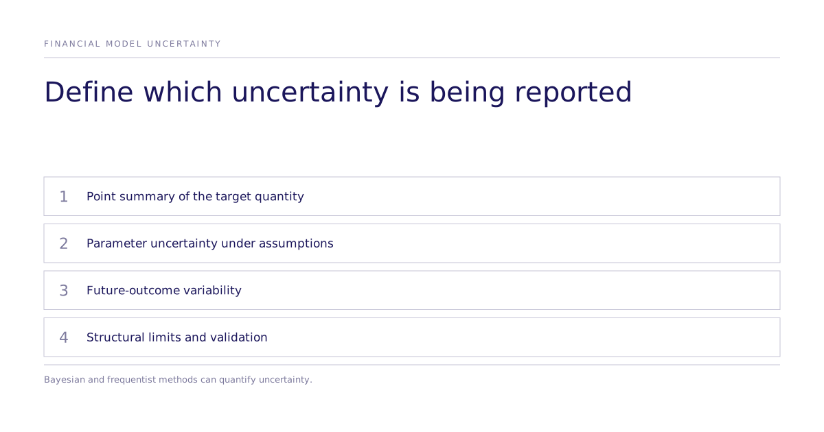
A financial-model buyer needs more than a point estimate of beta, loss, or option value: ask which uncertainty is quantified and which assumptions remain outside the calculation. Bayesian inference supplies a posterior conditional on a specified likelihood and priors. Frequentist methods also quantify uncertainty. Neither approach guarantees calibration or identifies every source of market risk.
Which assumptions matter for inference?
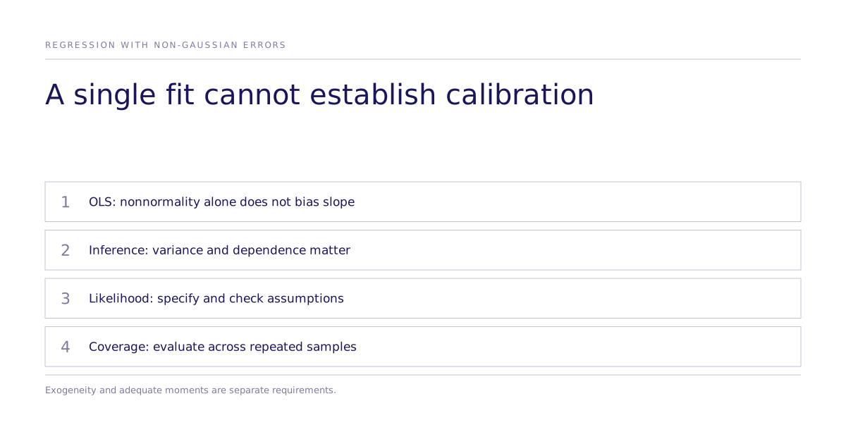
OLS coefficient fitting does not require Gaussian errors. Under appropriate exogeneity and finite-moment conditions, non-normality alone does not bias the slope. Exact small-sample Gaussian inference has additional assumptions. Heteroskedasticity, dependence, misspecification, and endogeneity require separate attention; covariance estimates allowing heteroskedasticity or dependence can address some inference issues, not all model errors (Statsmodels covariance estimators).
A Bayesian posterior represents parameter uncertainty within the specified model. It does not include every plausible model configuration or every omitted structural risk. Inspect likelihood, priors, sampling diagnostics, predictive checks, and sensitivity before relying on the distribution.
Quantifying uncertainty instead of picking one model
A frequentist beta estimate may come with a sampling-based confidence interval. A Bayesian beta posterior expresses uncertainty conditional on likelihood and priors. Predictive outcomes require an additional step that includes future observation variability. Compare both methods on held-out performance and coverage appropriate to the decision.
A narrow parameter interval can coexist with substantial future-return uncertainty. A mixture or changing-regime model can represent some structural variation, but a distribution over coefficients alone does not discover all regimes. Define the risk quantity before choosing a model.
How do you model errors that are not normally distributed?
PyMC Labs' June 27, 2025 finance article, by Camilo Saldarriaga, Alexander Fengler, and Jesse Grabowski, illustrates a regression with skewed, heavy-tailed errors. A fit displayed for one simulated dataset does not establish bias or interval coverage over repeated datasets. Use it as a qualitative illustration of likelihood choice. To claim calibration, provide the generator, sample size, priors, repetitions, interval definition, and observed coverage.
Both Bayesian and frequentist models can represent non-Gaussian outcomes. Select distributions from the data-generating assumptions and diagnostics. Compounded wealth is a product of gross returns; a lognormal form requires assumptions about the log-return sum. It is not a general property established by placing a lognormal prior on a parameter.
Value at risk and option pricing under full uncertainty
For value at risk, define the loss variable, horizon, and quantile. Distinguish a loss quantile conditional on a fitted model, a posterior distribution over that quantile, and a quantile of the posterior predictive loss distribution. They answer different questions. Tail shape, dependence, regime changes, and data coverage can matter more than the width of a parameter posterior.
For option valuation, a simulated payoff is not itself an option value. Under the specified risk-neutral pricing model, value is a discounted expected payoff. Repeating that valuation under uncertain parameters can produce uncertainty about the model value; it remains separate from realized payoff risk and from numerical Monte Carlo error. QuantLib's Monte Carlo European engine is one implementation reference.
Open-source tools such as PyMC make specified probabilistic models executable. Tool availability does not establish model adequacy, financial profitability, or a comparative adoption rate.
Where this connects to testing a market decision before it ships
A buyer-choice experiment addresses a different question from historical financial modeling: how a tested intervention changes a measured response under its design assumptions. Discuss a Subconscious study with its audience, comparator, assignment, endpoint, and uncertainty method. Generated choices do not establish what a target market actually buys. The public evidence record provides aggregate choice-parameter rank replication context rather than financial risk-model validation.
What are the limits of either approach?
Ask the vendor for source revisions, data availability, assumptions, reference calculations, sampling or numerical diagnostics, prior sensitivity where relevant, and held-out evaluation of the decision quantity. A credible interval describes uncertainty under a model; it does not repair endogeneity, missing regimes, or an incorrectly defined loss or valuation target.