Where Should the Next Wegmans Open? 7 Checks for a Bayesian Site-Selection Forecast
A new-store forecast should separate observed evidence from assumptions before a retail real estate team commits build-out and lease capital or accepts the risk that a new location will divert demand from nearby stores.
This guide draws on PyMC Labs' May 19, 2026 Wegmans site-selection account, written with Wegmans and PyMC Labs contributors. The case combines road access, demographics, analyst input, and probabilistic sales forecasts. Its store-count and opening-cadence descriptions are the case's planning context, rather than current delivery benchmarks.
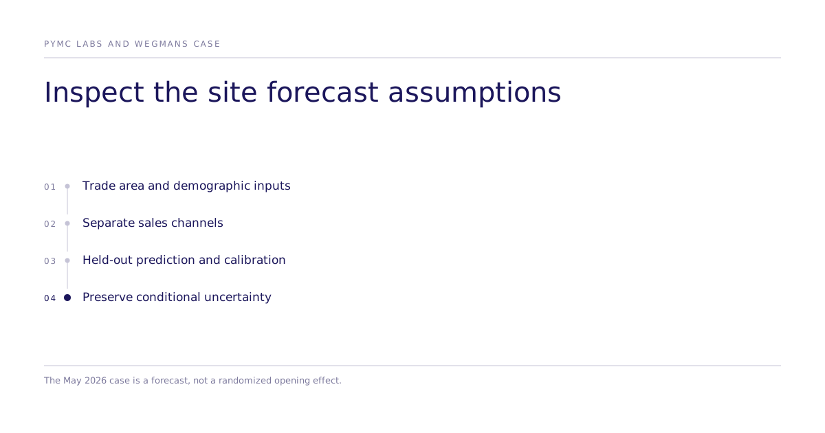
Use these seven checks to interrogate any comparable site forecast. Each check identifies an input, modeling choice, or judgment that a buyer should be able to inspect.
1. Define the trade area by travel time
A simple radius treats every direction as equally accessible. A road-network catchment instead reflects the routes people can use, including street layout and physical barriers. Travel-time isochrones estimate how far a customer can travel within a chosen interval, which is why they matter for catchment analysis at retail sites (TravelTime).
The team constructed a driving graph around each store from a roughly 20-mile buffer. Road classifications supplied edge speeds and travel-time values. A shortest-path calculation produced nested catchments from 2 minutes out to 24 minutes. When catchments overlapped, the location with the shorter trip received the contested area. A buyer should ask whether the network data, travel assumptions, and overlap rule match local shopping behavior.
2. Allocate demographics within partial boundaries
Census geography and a store catchment rarely share the same edges. Weighting a partially included block group only by land area can misrepresent where households actually sit, especially when settlement is concentrated in one corner.
The example addressed that mismatch with a quadkey tile grid and geocoded delivery-point density. The density inside each clipped block group determined how much of its population and household data contributed to the store profile. The buyer's check is straightforward: confirm that demographic allocation follows inhabited places rather than empty acreage.
3. How are store and ecommerce demand modeled separately?
The historical model estimated in-store and ecommerce sales through two distinct channels while sampling them together, so total demand carried uncertainty from both outcomes. It also let the model constrain coefficient direction where domain knowledge justified it and incorporate an analyst's ordered visibility assessment without pretending that judgment was a precise physical measurement.
Both sales outcomes used the trailing 52 weeks of data in the source setup. That was a historical modeling choice intended to reduce seasonal distortion, not a universal prescription. A buyer should inspect whether channel definitions, averaging windows, and judgment variables fit the decision now being made.
4. What does full-refit leave-one-out validation test?
With roughly 100 stores in the fitting data, the case describes full-refit leave-one-out validation: remove one store, refit, and predict the omitted observations. This evaluates the specified model's site predictions beyond its fitting observations. If model choices or weights are selected using those same results, request an additional untouched test where feasible, and assess whether nearby-store dependence or changing markets limit generalization.
The joint score evaluates the two observed sales channels together, but an aggregate can still conceal channel-specific weaknesses. Request separate residual, calibration, and predictive-interval coverage results for each channel and across relevant types of sites.
5. How is uncertainty preserved when combining models?
The example compared several model variants and assigned weights according to predictive fit. It then combined posterior samples using those weights rather than blending only the central forecasts. Keeping the samples preserves distribution shape and supports probability questions, such as whether sales clear a planning threshold.
This matters because a single expected value can hide asymmetric or multi-peaked risk. The useful buyer artifact is the range of plausible outcomes and the assumptions behind its shape, not merely the headline estimate.
6. Recalculate neighboring-store inputs
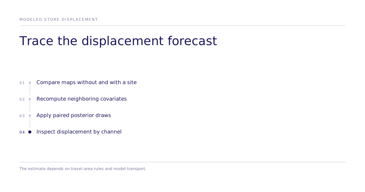
Adding a proposed site changes the modeled territory assigned to nearby stores. The case compares inputs without and with the candidate and applies paired posterior draws to the resulting covariates. This produces a conditional forecast of displacement by store and channel. It is not a randomized estimate of actual cannibalization: the result depends on the trade-area rule, sales model, and whether the relationship transports to a new opening.
The sequence is important: proposed site, revised trade areas, recomputed covariates, updated sales forecast, then estimated displacement. A buyer can trace that chain to identify where measured evidence ends and analyst judgment begins.
7. Keep the analyst in the decision loop
An analyst supplied a candidate address, square footage, parking type, visibility score, and operating zone. The interface returned expected weekly sales with an uncertainty interval, affected-store estimates by channel, and a map of the revised trade areas.
Those outputs informed a broader decision that still included market visits, competitive intelligence, and real estate judgment. The interface is useful when it exposes assumptions and uncertainty. It is dangerous when polished output encourages the team to treat the forecast as an automatic site decision.
The question that remains after the shortlist
These seven checks can improve confidence in how a site forecast was assembled. They do not establish which concept, assortment, or message will change behavior among shoppers in the selected trade area.
If the unresolved question concerns an assortment or message, design a separate study for that action and endpoint. A human task records stated responses; a simulated task records generated responses and needs matched validation. Keep population and intervention changes visible if a later live or human study follows. Read the aggregate validation evidence and CPG decision examples for scope.
Keep the boundary visible
The site-selection case forecasts sales and modeled neighboring-store displacement. A choice task answers a different question about responses to specified alternatives. Confirm the required spatial, commercial, technical, and human evidence with the project provider rather than infer a categorical product exclusion or a guaranteed handoff.
Bring the candidate sites, forecast assumptions, existing-store effects, and unresolved concept or message question to scope the next study.