Counterfactual Causal Inference in PyMC
Prediction forecasts the outcome under current conditions. Causal inference instead estimates the outcome that a different action would have produced.
That distinction changes how a team measures impact. After an illustrative $250,000 advertising campaign, observed sales alone cannot show how many sales the campaign caused. The missing quantity is the outcome in the same period without the campaign. That unobserved alternative is the counterfactual.
A Bayesian model can estimate the counterfactual as a distribution rather than a single guess. The difference between the observed outcome and that modeled baseline gives an estimate of the causal effect, subject to the assumptions in the model.
Excess deaths as a counterfactual problem
The same structure appears in public health. Excess deaths can be written as:
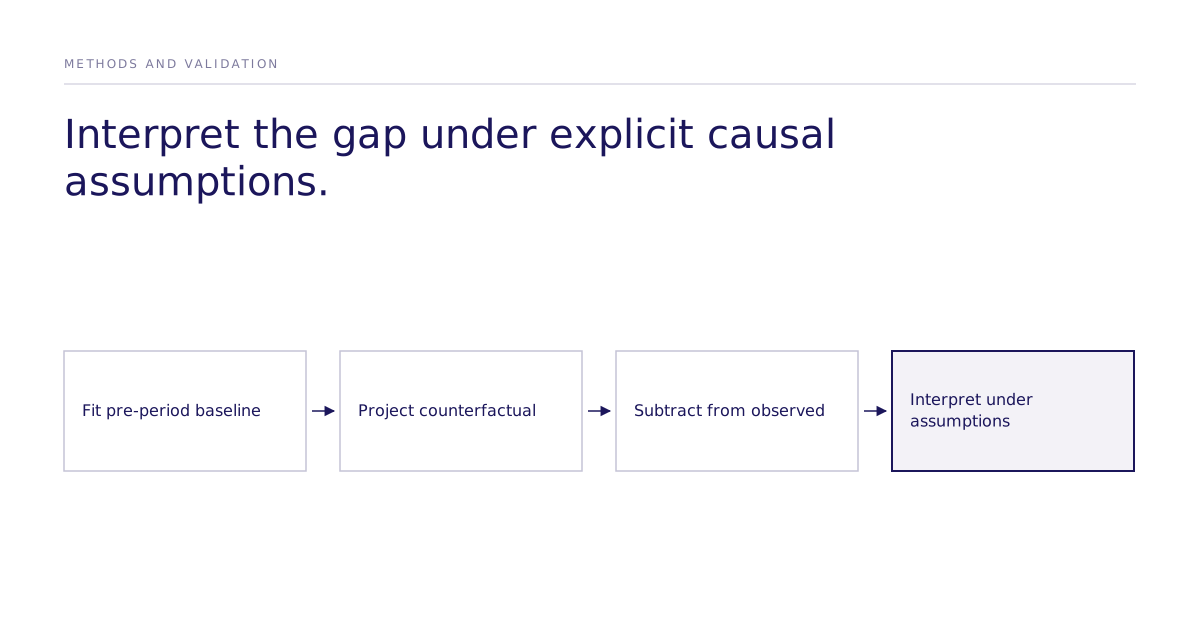
\text{Excess Deaths} = \text{Reported Deaths} - \text{Expected Deaths}Reported deaths are observed. Expected deaths in a world without COVID-19 are not. To estimate them, fit a model to the period before COVID-19, project the learned mortality pattern into the later period, and compare that projection with reported deaths.
The example uses monthly deaths in England and Wales. Mortality has a clear seasonal pattern, so a credible baseline must account for that pattern before it can attribute the remaining gap to the pandemic.

How do you make causal assumptions visible?
A directed acyclic graph, or DAG, forces the analyst to state which variables are treated as causes, proxies, or omitted factors.
The example models reported deaths using:
- Time, as a proxy for demographic aging
- Month, as an index for seasonal effects
- Temperature, as a direct influence on mortality
COVID-19 is deliberately left out of the baseline model. The purpose is to forecast a world where the pandemic did not occur. Adding a pandemic indicator would let the model explain the observed shock rather than estimate mortality in its absence.

This exclusion does not make the estimate causal by itself. The conclusion depends on assumptions: the pre-pandemic relationship remains useful in the later period, the selected predictors capture the important baseline structure, and no other unmodeled shock explains the observed difference.
Translate the DAG into a Bayesian model
Let monthly deaths be a function of time, month, and temperature:
\text{deaths}_t = f(\text{time}_t, \text{month}_t, \text{temp}_t)Here t runs from 1 through T.
Linear baseline specification
A linear specification is:
f(\text{time}_t, \text{month}_t, \text{temp}_t) =
\beta_0 + \beta_1\text{time}_t + \beta_2\text{temp}_t + \vec{s}[\text{month}_t]
Specify priors and likelihood
The vector s contains 12 monthly effects. The notebook uses a zero-sum seasonal construction. Its priors and likelihood can be summarized as:
\begin{aligned}
\beta_0 &\sim \text{Normal}(40000, 10000)\\
\beta_1 &\sim \text{Normal}_+(0, 50)\\
\beta_2 &\sim \text{Normal}(0, 200)\\
\vec{s} &\sim \text{ZeroSumNormal}(3000), \quad \sum_{m=1}^{12}s_m=0\\
\mu_t &= \beta_0 + \beta_1\text{time}_t + \beta_2\text{temperature}_t + \vec{s}[\text{month}_t]\\
\sigma &\sim \text{HalfNormal}(2000)\\
\text{deaths}_t &\sim \text{Normal}_+(\mu_t, \sigma)
\end{aligned}
The notebook constructs 12 monthly effects from 11 unconstrained Gaussian coordinates. Their sum is zero, separating seasonal deviations from the intercept; the monthly effects are not 12 independent Normal draws. This constraint follows the PyMC excess-deaths notebook, accessed October 2, 2026.
These priors translate directly into modeling choices:
- β₀, Normal(40000, 10000): the intercept, centered at 40,000 monthly deaths
- β₁, Normal₊(0, 50): the time trend, constrained positive for an expected upward trend in the susceptible population
- β₂, Normal(0, 200): the temperature effect, which can move the estimate in either direction
- σ, HalfNormal(2000): the noise scale
Check the model before asking for an effect
Counterfactual inference is only as useful as its baseline. Bayesian workflow provides several checks before the final comparison.
Prior predictive check
Draw outcomes from the model before conditioning on observed deaths. The prior predictive distribution reveals whether the model permits plausible mortality levels and seasonal variation.
The example inspects 50% and 95% credible regions. If those ranges miss plausible values before the model sees data, the priors or functional form need work.

Fit only the pre-intervention period
Posterior sampling uses pre-COVID observations. This prevents the pandemic shock from changing the coefficients used to define the no-pandemic baseline.
Check posterior predictions in the fitted period
Compare observed pre-COVID deaths with posterior predictive draws. A model that cannot reproduce the baseline period should not be trusted to project its counterfactual into a new period.
Good fit is necessary but not sufficient. A flexible time-series model may predict well while relying on a causal story that fails under intervention.
Generate the counterfactual with pm.set_data()
The following is a code fragment, not a standalone script. It assumes the notebook has defined the fitted model, posterior idata, mutable inputs named month, time and temp, an observed variable named obs, and aligned post-period arrays.
After fitting the model, replace its time, month, and temperature inputs with their post-COVID values while keeping draws from the fitted parameter posterior. Then sample the posterior predictive distribution:
with model:
    pm.set_data({
        "month": month_post,
        "time": time_post,
        "temp": temp_post,
    })
    counterfactual = pm.sample_posterior_predictive(
        idata,
        var_names=["obs"],
    )
This operation produces simulated post-COVID deaths, including observation noise, under the fitted no-pandemic model. It is often described with the do-operator:
P(\text{deaths} \mid \vec{\beta}, \vec{s}, \sigma,
\text{do}(\text{time}=\mathbf{t}, \text{month}=\mathbf{m},
\text{temp}=\mathbf{temp}))
Identification assumptions
Whether that distribution identifies a causal effect still depends on the DAG and the stability assumptions. pm.set_data() is a computational mechanism, not a substitute for causal identification.
How do you calculate and interpret the effect?
For each posterior draw, subtract the sampled post-COVID deaths (which include observation noise, not just the mean) from reported deaths. The resulting distribution represents monthly excess deaths under the model. Summing across months produces cumulative excess deaths while retaining posterior uncertainty.
The original analysis displays 50% and 95% credible regions for the expected and excess-death estimates. That is more informative than a single total, but the bands quantify parameter and sampling uncertainty conditional on the specification being correct; they do not capture the trend-extrapolation and misspecification risk of projecting a linear trend roughly two years past the fitting window.

The gap may include both direct deaths from COVID-19 and indirect effects, such as disrupted access to care. The model estimates the effect of the pandemic period as represented by the design, not every mechanism inside it.
Apply the same structure to business decisions
The mortality example maps cleanly to commercial questions:
- Sales with a campaign versus expected sales without it
- Conversion after a price change versus expected conversion at the prior price
- Retention after a product change versus expected retention without the change
- Learning after an intervention versus expected learning without it
Each application needs more than a before-and-after chart. Specify the intervention, draw the causal graph, define the pre-intervention baseline, test predictive adequacy, and state the assumptions required to interpret the difference as causal.
The full PyMC notebook, pm.set_data() documentation, and pm.sample_posterior_predictive() documentation provide the implementation details.
Relate counterfactual modeling to simulated choice
A counterfactual mortality baseline and a simulated choice experiment answer different questions. The former projects an observational baseline under explicit stability assumptions. The latter estimates assigned contrasts inside a configured model, with generated outcomes representing modeled stated choices. Neither supplies evidence of live-market transfer without a matched comparison.
Use the methods hub and simulation comparison guide to distinguish estimation, identification and validation. For either approach, report the intervention, assumptions, endpoint and uncertainty before recommending an action.